A knowledge guide from overview to detail: production systems, water quality, equipment, species, biology, economics, operations and automation - so you can move from a general question to deeper knowledge.
Missing something or have ideas? Contact us - we welcome constructive feedback. contact@dabce.se
Water Helper - water treatment
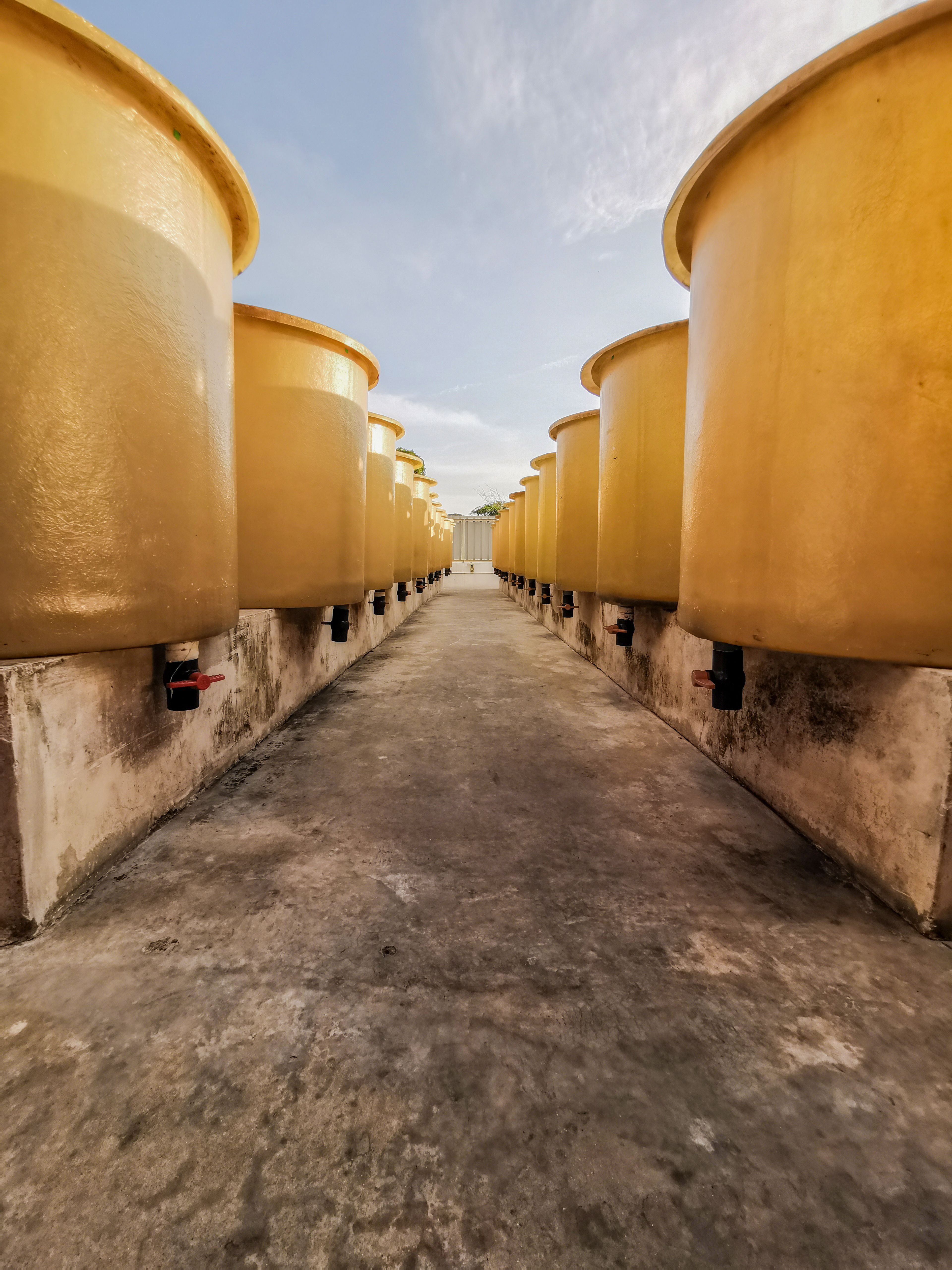
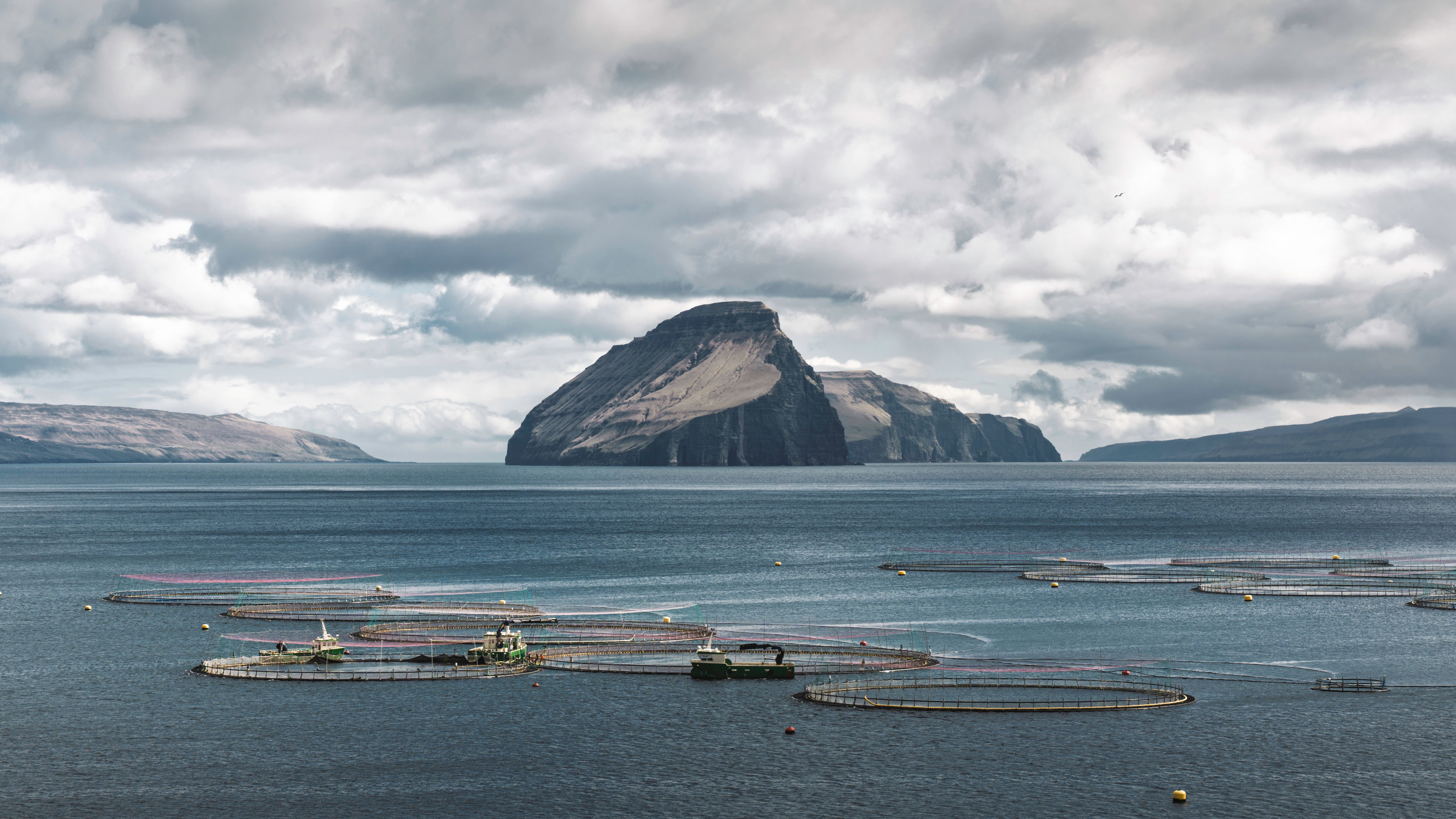

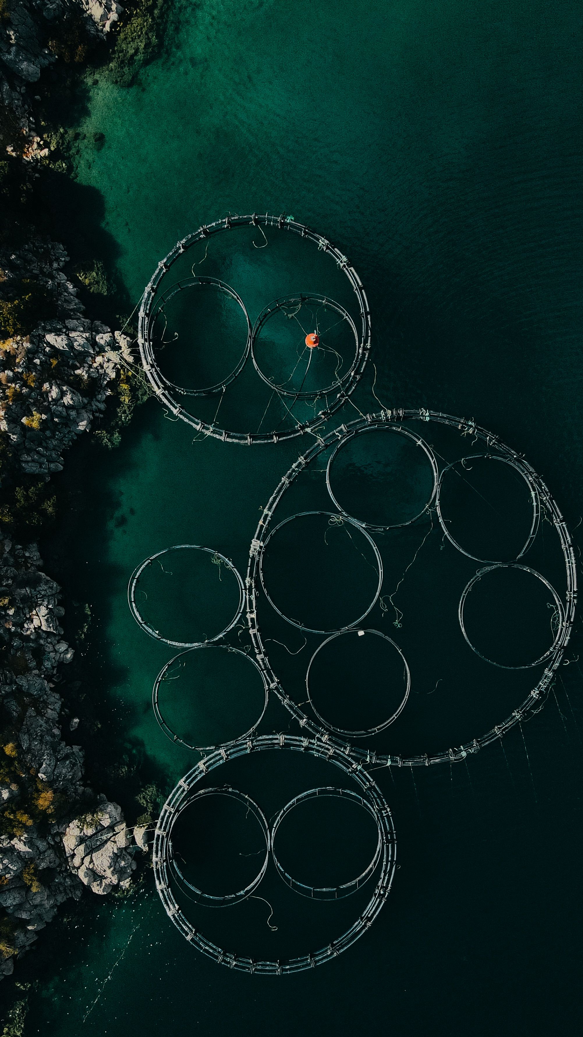
Images: land tanks, sea pens, pond culture and coastal farming
Pick a subject in the overview. Start broad and go deeper in each section. For concept sizing of land-based salmonid farms, see the FlowFarm model under Flow-Through Systems.
Aquaculture is the farming of aquatic organisms - fish, shellfish, algae and aquatic plants - under controlled or semi-controlled conditions. Unlike capture fisheries, growth, feed, water quality and harvest are managed by the farmer.
Aquaculture can be practised in freshwater, brackish water or seawater depending on species requirements and local conditions. Fish and shellfish can be farmed directly in natural waters - for example in cages placed in lakes, fjords, rivers or coastal waters. Farming can also take place in land-based facilities.
Traditionally many farms have been flow-through systems where water is taken from a nearby watercourse through ponds, raceways or culture channels before being returned to the environment. Modern aquaculture also includes recirculating aquaculture systems (RAS), where water is reused and treated in several stages with mechanical filters, biological treatment, degassing, UV or ozone. By controlling water quality, the farmer can create optimal conditions for fish growth while reducing water use and environmental impact.
Aquaculture is today the fastest-growing sector in food production and has become a central part of the world supply of fish and shellfish. According to the Food and Agriculture Organization of the United Nations (FAO), about 141 million tonnes of aquaculture products were produced globally in 2024, including fish, shellfish, crustaceans, algae and seaweeds. Of this, just over 100 million tonnes were farmed aquatic animals such as fish, shrimp and mussels. Aquaculture now accounts for more than half of world production of aquatic animals and is therefore one of the most important protein sources for a growing global population.
Asia dominates global volume. China is the world's largest producer with extensive freshwater and coastal culture (fish, shrimp, mussels, algae). Southeast Asia (e.g. Vietnam, Indonesia, Thailand) is strong in shrimp, pangasius and other warm-water species. India is growing fast in freshwater aquaculture and shrimp. Japan and Korea combine advanced technology with premium species, often in smaller high-value systems. Africa has large potential and expanding pond and tilapia culture, though infrastructure and feed chains vary widely between countries. North America combines traditional farming with investment in land-based salmonids (RAS). South America - especially Chile - is a powerhouse in cage salmon, with growing focus on technology and sustainability. Western Europe and the UK mix cage, raceway and land-based projects; Eastern Europe has ponds, pike-perch/perch and rising interest in modern systems. In the Nordic countries, cage farming is strong in Norway, while Sweden, Finland and other inland settings more often work with rainbow trout, Arctic char and land-based or semi-land-based systems - raceways, semi-flow-through and RAS.
See also the sections on production systems and species, and our DABCE FlowFarm model for concept sizing.
Aquaculture offers several major advantages for food systems, the environment and regional development. It can supply protein at industrial scale without increasing catch from already pressured wild stocks, and it can be located where markets, power and skills exist - including close to the consumer.
Land-based and semi-land-based farms can be located near cities, logistics hubs and power grids. That shortens transport chains, improves traceability and often strengthens the local economy (jobs, suppliers, services). It aligns with the UN Sustainable Development Goals, including SDG 2 (zero hunger) via more access to nutritious food, SDG 8 (decent work and economic growth) via green industry and jobs, and SDG 12 (responsible consumption and production) via more controlled flows and traceability.
When wild stocks are limited or overfished, farming can add volume without increasing fishing pressure in seas and lakes. Aquaculture does not replace responsible fisheries management, but it can close the gap between demand for fish and what sustainable fishing can supply - supporting food security and reduced hunger (SDG 2) as well as life below water (SDG 14).
More advanced systems - especially RAS and well-designed semi-flow-through - make it possible to treat and control water quality in ways traditional open-water cage farming cannot. Solids, nutrients and organics can be captured and treated before discharge; oxygen, CO2 and temperature can be held within good limits. The result can be lower load on the receiving water, more predictable water quality in the farm, and better conditions for fish health and welfare than production that relies only on the surrounding water body.
Aquaculture is not a modern invention. Already more than 4,000-5,000 years ago there is evidence that people actively held and harvested fish in constructed water systems - long before industrial feed, hatcheries and RAS.
In ancient Egypt, tomb paintings and reliefs show fish held and taken in constructed ponds and garden pools along the Nile - early pond culture rather than today's floating net pens. The literature often cites evidence around 2500 BCE (over 4,500 years ago) for built ponds, and more widely accepted scenes of line-fishing for tilapia in irrigated ponds around 2000-1500 BCE. Nile tilapia (Oreochromis niloticus) recurs in art and had its own hieroglyph. (See e.g. the review by Rogers 2024, Journal of Archaeological Research, citing Balarin & Hatton 1979; Brewer & Friedman 1989; Nash 2011; Costa-Pierce 1987.)
In China, archaeology points to even older roots. At the Early Neolithic site of Jiahu (Henan), body-length distributions of carp remains have been interpreted as early managed carp culture/water-level control around 6200-5700 BCE - about 8,000 years ago, contemporary with early rice farming and water management (Nakajima et al. 2019, Nature Ecology & Evolution: "Common carp aquaculture in Neolithic China dates back 8,000 years"). Later written sources include Shang-period oracle bones on fishing in garden ponds and Fan Li's carp-culture treatise (Yang Yu Jing) from about the 5th century BCE.
Pond culture then spread and was refined across Europe and Asia over the centuries. Modern aquaculture accelerated in the 20th century with dry feeds, hatchery methods, cages and later RAS.
Rainbow trout and Atlantic salmon became global industrial species. In the Nordic countries, inland farming grew with raceways and ponds while cages dominated in Norway. Land-based post-smolt and food-fish RAS now drive a new investment wave.
Sources (selection): Nakajima et al. (2019), Nature Ecology & Evolution 3:1415-1418 - Jiahu/carp; Rogers (2024), J. Archaeol. Res. - review of ancient aquaculture incl. Egypt; Nash, C.E. (2011), The History of Aquaculture (Wiley-Blackwell); Costa-Pierce, B.A. (1987), Aquaculture 63:321-337 - early Egypt/tilapia.
Aquaculture is one of the fastest-growing food production sectors in the world and now provides more than half of all aquatic animal products consumed by humans. Global production continues to increase as wild fisheries have reached biological and practical limits, making aquaculture essential for future food security. According to the FAO, aquaculture has surpassed capture fisheries as the primary source of aquatic animals for human consumption and is expected to play an even larger role in supplying protein to a growing global population.
Asia dominates production volumes, accounting for the vast majority of global aquaculture output, with China, India, Indonesia, Vietnam and Bangladesh among the leading producers. Europe and North America, while representing a smaller share of total volume, lead in high-value species such as Atlantic salmon, Arctic char, trout and marine finfish. These regions are also global centres for advanced aquaculture technology, including recirculating aquaculture systems (RAS), water treatment solutions, oxygenation systems, digital monitoring, automation and artificial intelligence.
Industry profitability is driven by a combination of biological performance and operational efficiency. Key factors include feed conversion ratio (FCR), energy costs, fish survival rates, growth performance, market pricing, financing conditions and regulatory permitting processes. As modern facilities become increasingly technology-intensive, operational excellence and resource efficiency are becoming major competitive advantages.
A rapidly growing segment of the aquaculture value chain is the technology supplier ecosystem. Companies providing water treatment, oxygen generation, ozone systems, UV disinfection, filtration, sensors, automation, digital twins and AI-driven decision support are experiencing strong demand as producers seek higher productivity, lower environmental impact and improved regulatory compliance. Technology exports have therefore become a strategic industry in their own right, supporting aquaculture development globally - including from the Nordic countries.
Long-term growth is expected to be driven by increasing demand for sustainable protein, pressure on wild fish stocks, urbanization, stricter environmental regulations and continuing advances in land-based farming and precision aquaculture technologies. These trends are creating opportunities not only for fish producers but also for engineering, water treatment and digital infrastructure companies serving the sector.
Million tonnes (live weight)
Aggregated from FAO Global production (FishStat): aquaculture = freshwater+brackish+marine; capture = capture. Yearbook group "Fish, crustaceans and molluscs, etc." only (excludes algae, mammals, corals, etc.).
Compare SOFIA 2024: 2022 was the first year aquaculture surpassed capture for aquatic animals (~94 Mt vs ~91 Mt).
Source: FAO. Global production quantity statistics (FishStat / GlobalProduction dataset). https://www.fao.org/fishery/en/statistics/software/fishstatj · Licence: FAO Fishery datasets: CC BY-NC-SA 3.0 IGO (see FAO dataset terms). Chart prepared by DABCE for educational knowledge use with attribution. · Chart: DABCE · 2026-08-09
After the Second World War, population and demand for protein rose. From the 1960s to the 1980s industrial capture fisheries expanded with larger vessels, more efficient gear and greater range. FAO time series then show global capture volumes of aquatic animals largely levelling off, while aquaculture continues to grow. According to SOFIA 2024, aquaculture first surpassed capture fisheries in aquatic-animal production in 2022. That plateau is commonly interpreted in research and FAO reports as many fisheries approaching biological and management limits while demand for aquatic protein keeps rising.
In many fisheries the composition of the catch has changed over time - including use of more species and size classes - while management, quotas and technology have evolved. Aquaculture complements capture fisheries by adding farmed volume under controlled conditions. It does not replace responsible stock management, but can support food supply when wild catch can no longer grow at the same pace. Land-based and semi-land-based systems are also part of EU and national strategies for a sustainable blue economy, alongside sustainable fisheries.
Recirculating Aquaculture Systems (RAS) are among the fastest-growing segments of the industry. By continuously treating and reusing water, RAS facilities can reduce freshwater consumption by more than 95%, enable production closer to consumers, improve biosecurity and support sustainable growth in regions where traditional net-pen farming is limited. This has created substantial demand for advanced filtration, oxygenation, monitoring and water treatment technologies - areas where DABCE and similar technology suppliers operate. See also the RAS section and our DABCE FlowFarm model for concept sizing.
Modern aquaculture can be divided into two main production models: land-based systems and sea/lake-based systems. Each approach has distinct advantages, challenges and environmental considerations. The choice depends on species, location, regulations, water availability, logistics and investment strategy.
Land-based facilities raise fish in tanks located indoors or outdoors on land. Most modern facilities use Recirculating Aquaculture Systems (RAS), where water is continuously filtered, treated and reused.

Typical species include Atlantic salmon, rainbow trout, Arctic char, sturgeon, shrimp, eel and various hatchery-produced marine species.
Net-pen farming uses cages installed in oceans, fjords, bays or freshwater lakes. Fish grow in natural water bodies while operators provide feed, monitoring and husbandry.
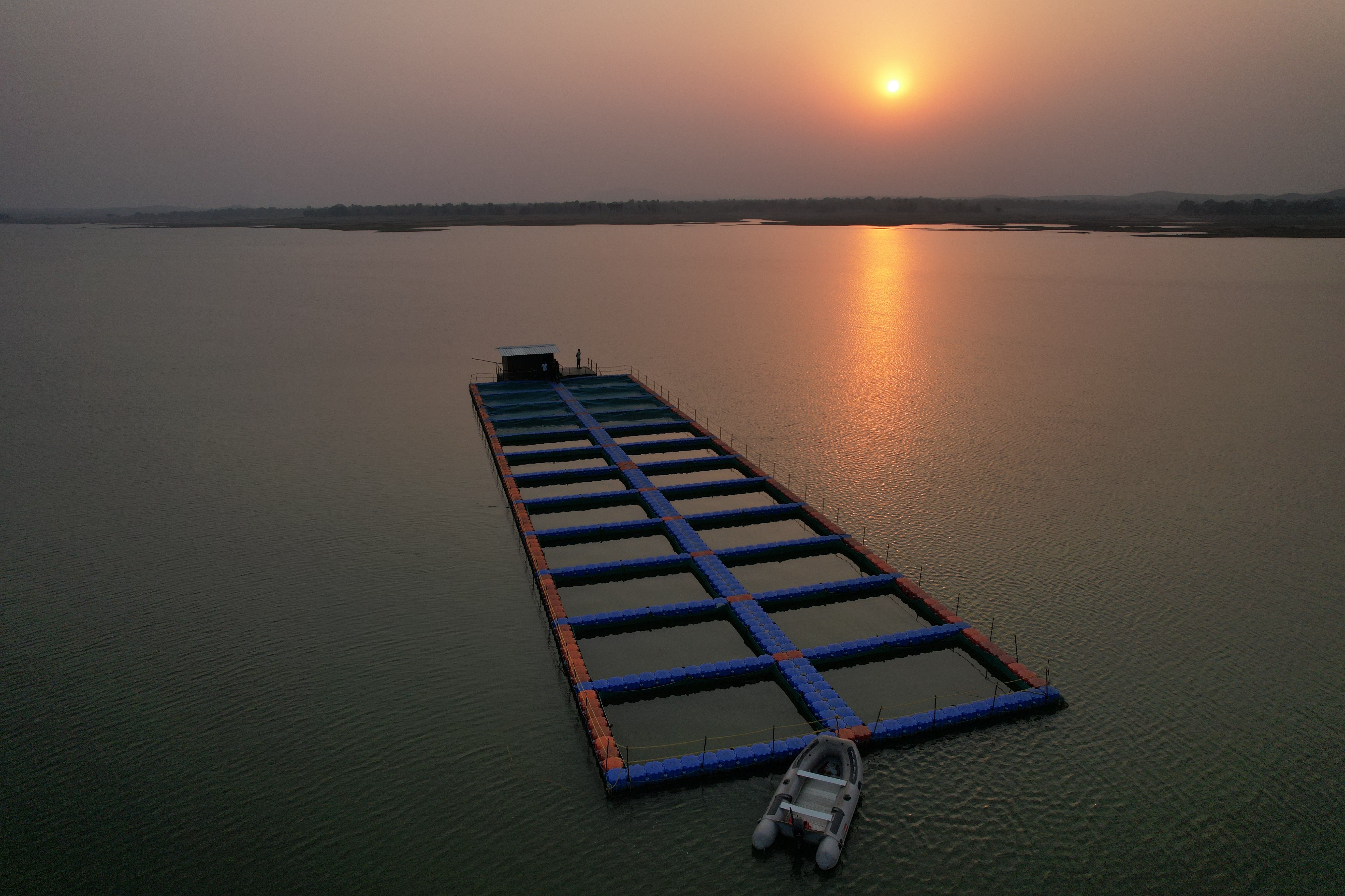
Net-pen systems are widely used for salmon, trout, sea bass, sea bream and many other marine species.
Earthen and lined ponds are a third, very widespread form - often on land but at lower technical intensity than RAS. They dominate volume in parts of Asia, Africa and Latin America, while Europe and North America more often use raceways, net pens and land-based systems.
Land-based RAS facilities are expanding rapidly in regions where environmental regulations, biosecurity requirements, freshwater scarcity or market proximity favour controlled production. However, sea-based net-pen farming still accounts for the majority of global salmon production due to its lower production cost and large-scale operational maturity. Hybrid and semi-flow-through solutions (e.g. land-based start with strong treatment) often bridge the two models. See also the RAS section and our DABCE FlowFarm model for concept sizing.
The future of aquaculture is shaped by food demand, environmental requirements, technology and geography. Wild fisheries often cannot grow at the same pace as demand; at the same time societies want more traceable, local and controlled production. That drives investment in land-based systems, better water treatment, digital operations and circular flows - not least in Europe and the Nordic countries.
Land-based RAS and semi-flow-through grow where permits, biosecurity or market proximity favour controlled culture. Precision tools - sensors, automation, AI for feeding and biomass, digital twins - reduce risk and improve FCR and energy use. Hybrid models (hatchery and juveniles on land, on-growing in cages or the reverse) remain important where they deliver the best economics and lower environmental risk.
Feed remains the large environmental and cost factor. Future feeds mix more alternative proteins and oils, while culture of herbivorous and omnivorous species can reduce dependence on fishmeal. Technology export - water treatment, oxygen, UV/ozone, monitoring - becomes a growth engine beside fish production itself.
The future of aquaculture may not consist of isolated farms producing a single species. Instead, future systems could become highly integrated biological ecosystems where nutrients, carbon and energy are continuously recycled between multiple organisms.
Microalgae and macroalgae (seaweed/kelp) are expected to play a central role. Using sunlight or renewable energy, algae can convert carbon dioxide and nutrients into valuable biomass rich in proteins, oils, vitamins and minerals. This biomass can then serve as feed for the next level of the food chain.
Crustaceans such as shrimp, freshwater prawns and certain filter-feeding species can utilise algae-derived feeds, while herbivorous and omnivorous fish species such as carp, tilapia and some catfish can efficiently convert plant-based ingredients into high-quality animal protein. Because these species are lower on the food chain, they generally require less feed input than carnivorous fish.
Predatory fish species such as salmon, trout, sea bass and tuna occupy higher trophic levels and require greater amounts of protein and energy. Future feed technologies may reduce reliance on wild fish resources by using ingredients derived from algae, insects, microbial protein and circular agriculture systems.
In the most advanced concepts, waste streams become resources. Fish waste and uneaten feed can be processed into fertiliser, biogas or nutrient concentrates. These nutrients can then support algae cultivation, hydroponic crops, aquatic plants and kelp production, creating a circular industrial ecosystem with minimal waste.
Sunlight / renewable energy
⬇️
Algae & kelp
⬇️
Crustaceans & insects
⬇️
Herbivorous & omnivorous fish (carp, tilapia)
⬇️
Carnivorous fish (salmon, trout, sea bass)
⬇️
Nutrients, sludge & organic residues
⬇️
Algae & kelp (recirculation)
Looking forward: Future aquaculture may increasingly resemble natural ecosystems, where nutrients continuously cycle through algae, plants, crustaceans, fish and microbial communities. Such systems could maximise food production while minimising freshwater use, waste generation and environmental impact. On Earth these closed-loop systems may improve sustainability and resource efficiency. In the future, similar concepts could support permanent human settlements on the Moon, Mars and beyond, where every litre of water and every gram of nutrients must be reused.
It may sound like science fiction, but aquaculture could become an important part of future food production in space. As humanity moves toward long-duration missions, lunar bases, and eventually settlements on Mars, astronauts will need reliable sources of fresh food that can be produced using limited water, energy and resources.
The first step will likely be algae cultivation. Microalgae grow quickly, require little space, consume carbon dioxide, and can produce proteins, vitamins, healthy fats and even oxygen. In many proposed life-support systems, algae are expected to play a key role in recycling nutrients and supporting human habitats.
As space agriculture becomes more advanced, aquaculture could expand beyond algae. Herbivorous and omnivorous fish such as carp may become attractive candidates because they efficiently convert plant-based feeds into high-quality protein. Unlike carnivorous fish that require feed made from other fish, carp can thrive on algae, aquatic plants, insects and other renewable food sources that could potentially be produced within a closed-loop space ecosystem.
Future space farms may combine hydroponics, algae cultivation, insect production and fish farming into a single integrated food system. Nutrients from fish waste could fertilise crops, while plants and algae help clean and recycle water. Such circular systems could dramatically reduce the need for resupply from Earth.
Fun fact: If humans establish permanent settlements on the Moon or Mars, one of the first farmed fish species may not be salmon or tuna, but humble carp. Their resilience, flexible diet and efficient growth could make them ideal "space fish" for feeding future explorers.
Perhaps one day, recirculating aquaculture systems (RAS) will not only produce fish on Earth but also support human settlements millions of kilometres away. The future of aquaculture may be truly out of this world - from FlowFarm on Earth to closed loops in space. The technology we develop now - water treatment, gas balance, monitoring and circular flows - is the same set of building blocks.
Not an official standard, just DABCE having a little fun. But there is a serious point behind it: whether supporting fish on Earth, a habitat on Mars, or a future station beyond the Kuiper Belt, the challenge is fundamentally the same. Build systems that recycle water, recover nutrients, minimise waste and keep life thriving in a closed loop. ♻️
| Domain | ARL / status |
|---|---|
| Aquaculture (commercial) | Commercially mature |
| RAS / land-based | Industrially scaling |
| Circular multi-trophic systems | Demonstration & pilot |
| FlowFarm concept (DABCE) | Concept & RFQ support |
| Destination | ARL / status |
|---|---|
| Moon | Early concepts and research |
| Mars | Future deployment candidate |
| Asteroid Belt | Long-duration habitat support |
| Kuiper Belt | Closed-loop civilization infrastructure |
| Interstellar | Carp status: under evaluation |
ARL = Aquaculture Readiness Level. Earth: serious status. Space: vision - with carp as the favourite "space fish" candidate.
Many people imagine fish farming as cages in the ocean or ponds in the countryside. In reality, some of the world's most advanced fish farms look more like water treatment plants, food factories, or even spacecraft life-support systems.
At its core, a Recirculating Aquaculture System (RAS) is surprisingly easy to understand. Think about a home aquarium. Fish swim in the tank and produce waste. Uneaten feed and feces accumulate. A filter removes particles and beneficial bacteria convert toxic ammonia into less harmful compounds. Air stones add oxygen, and from time to time water is replaced.
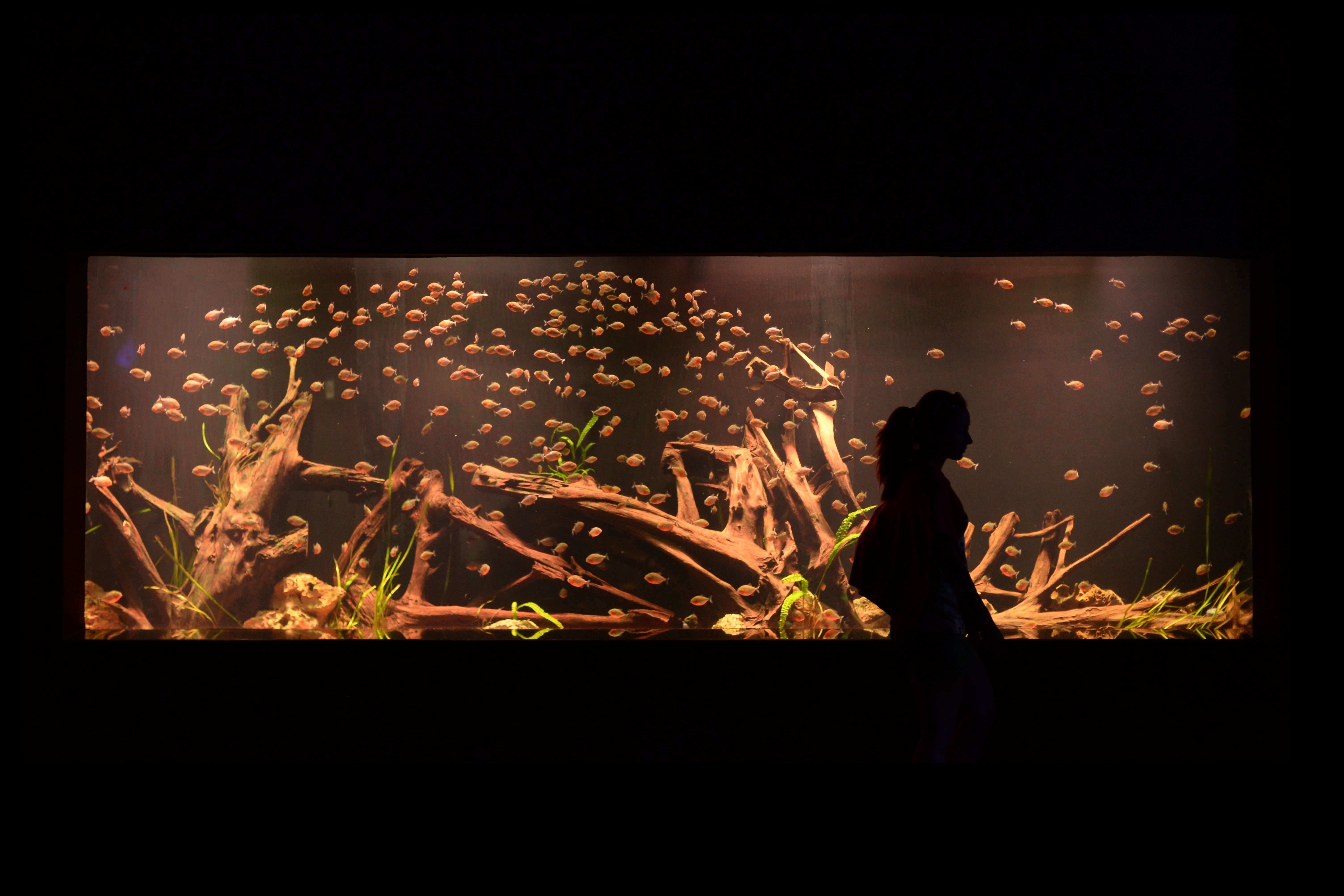
A RAS facility follows exactly the same principles, just on a much larger scale. Instead of a 200-litre aquarium, a commercial farm may contain millions of litres of water and thousands of tonnes of fish. Massive filtration systems, biofilters, oxygen generators and control systems continuously maintain water quality so the same water can be reused over and over again. In a traditional fish farm, water is used once and discharged. In a RAS facility, the water becomes a valuable resource that is treated, recovered and reused.
Fish do not consume water. They live in it. The challenge is keeping the water clean enough for the fish to thrive. Every kilogram of feed added to a fish tank eventually becomes: fish growth, carbon dioxide, ammonia, suspended solids and dissolved nutrients. A RAS system continuously removes or transforms these waste products so the water can return to the fish tanks. The result is that modern RAS farms may reuse more than 95% and in some cases more than 99% of their water while maintaining excellent environmental control.
Fish tanks
↓
Mechanical filtration
(drum filter / disc filter)
↓
Biofilter
(MBBR, fixed bed, biosand filter,
MBR, algae-producing unit / photobioreactor)
↓
CO2 removal
(degasser)
↓
Oxygen addition
(oxygen cone / LHO, aerators,
trickling filters, etc.)
↓
Microbiological control / sterilisation
(UV, ozone, etc.)
↓
Pump
↓
Back to fish tanks
+
Small make-up water stream
&
effluent treatment
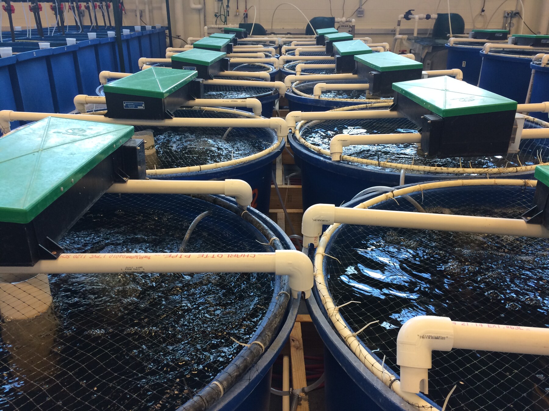
Not all RAS systems are the same. The simplest systems are often used for hatcheries, research facilities or small farms. These systems may exchange 10-30% of the water each day and rely heavily on incoming freshwater.
Many small trout hatcheries and fish research stations operate in this way. Think of it as a large aquarium with a generous flow-through component.
This is where much of today's commercial RAS industry operates. Water reuse typically ranges from 90-98%. These farms include drum filters, biofilters, degassers, oxygen systems and advanced monitoring.
Most modern land-based salmon, trout, Arctic char, eel and sturgeon facilities fall into this category. For many species and locations, this balance provides the best combination of economics, performance and operational reliability.
As water reuse increases, engineering becomes more demanding. At reuse levels above roughly 99%, almost everything that accumulates in water becomes important: carbon dioxide, fine particles, nitrogen compounds, dissolved organics, salts, microbial populations and trace elements. At this stage, the system behaves less like a fish farm and more like an industrial ecosystem.
Additional technologies may include ozone treatment, foam fractionation, membrane filtration, advanced oxidation, nutrient recovery, CO2 management systems and automated water chemistry control. These facilities can produce very large amounts of fish while using surprisingly little freshwater.
The future may push RAS even further. Instead of viewing waste as a problem, future systems may treat every output as a resource - for example feed for algae, crustaceans and omnivorous fish, while nutrients return into the system. Seaweed and kelp may become part of the cycle. Such systems begin to resemble natural ecosystems where nutrients flow through multiple organisms rather than being discarded. See also circular food ecosystems under future of aquaculture.
Fish
⬇
Nutrients & organic matter
⬇
Algae production
⬇
Shrimp, prawns & crustaceans
⬇
Omnivorous fish (carp, tilapia)
⬇
Carnivorous fish (salmon, trout)
⬇
Nutrients recovered back into the system
A major advantage of land-based RAS is biosecurity. In sea cages, fish are exposed to parasites, disease organisms, harmful algae, storms, predators and escapes. In a RAS facility, water conditions can be tightly controlled and external biological threats greatly reduced. This level of control is one reason why land-based production continues to grow globally.
The trade-off for all this control is energy. Energy is typically used for: pumping water, oxygen generation, heating or cooling, ventilation, UV systems, ozone generation, monitoring and automation. In cold climates, heating can dominate energy use. In warm climates, cooling may be equally important. As facilities become larger, even small improvements in pumping efficiency, oxygen transfer efficiency or hydraulic design can save substantial operating costs. Maximising air-side oxygen uptake in degassers and choosing the right total ΔDO cuts both flow and power - see our DABCE FlowFarm model for concept sizing.
A home aquarium might recycle a few hundred litres of water. A commercial RAS facility may recycle millions of litres every day. The underlying principle, however, is the same: keep the fish comfortable, keep the water clean, and continuously recycle valuable resources. That simple idea has evolved from the household aquarium into one of the most important technologies for future sustainable seafood production.
Flow-through is the classic land-based farming model: fresh water is taken from a source (river, lake, spring or well), passed through culture units - often raceways, concrete channels, ponds or tanks - and returned to the receiving water after more or less treatment. Unlike full RAS, only a small share of the water is reused (or none at all); oxygen and water quality in the farm are driven mainly by the incoming flow and how long the water stays with the fish.
The principle is simple and robust. Where water rights, source quality and the receiving water allow, flow-through has long been the standard for e.g. rainbow trout, smolt and other salmonids in cool freshwater. The site does not need the heavy pumping, filtration and oxygen infrastructure of a high-reuse RAS. The trade-off is high freshwater use, and nutrient, solids and sometimes pathogen discharges that must fit permits and the capacity of the receiving water.
In many parts of the world where aquaculture has grown faster than environmental regulation, this has led to significant local and regional environmental challenges. Eutrophication, oxygen depletion, sediment impacts and competition for water resources are examples of effects observed around intensive production areas. In water-stressed regions, large abstractions can also reduce water available to downstream users, agriculture and natural ecosystems.
As water becomes an ever more valuable resource and environmental requirements tighten, interest grows in technologies that cut both water use and discharges. This is a major driver behind modern RAS facilities and other high-reuse concepts. By treating and reusing water, production can be decoupled from large abstractions while nutrients and organic matter can be collected and treated in a more controlled way.
Water source
(river / lake / spring / well)
↓
Intake & coarse screening
(screens, trash racks, sometimes settling)
↓
Culture units
(raceways / tanks / ponds)
↓
Limited treatment
(settling, solids removal,
sometimes biofilter / polish)
↓
Discharge to receiving water
+
Optional partial return pumping
(semi-flow-through / PRAS)
Sizing starts from biomass, feed load and the water quality you need in the tank - above all dissolved oxygen, temperature, ammonia/TAN and solids. In pure flow-through, flow is the main lever: more water means more oxygen and more dilution of waste. That makes the farm sensitive to source flow, temperature and seasonal variation. In drought, ice runs or heat waves, capacity can fall quickly unless there is buffer volume, oxygen addition or scope to cut feed and biomass.
Even "simple" flow-through often needs solids removal and sometimes nutrient reduction under modern permits. Common steps are settling basins, microscreens, sludge thickening and in some cases biofilters or wetlands on the effluent. The tighter the permit and the more sensitive the receiver, the more the farm looks like semi-flow-through: more treatment, more reuse, more control - but still with a clear make-up stream from nature.
Many farms sit on a spectrum. Pure flow-through: almost all water passes once. Partial reuse (PRAS) / semi-flow-through: part of the flow is treated and returned, while a make-up stream brings in fresh water and a matching stream goes to the receiver after polish. That cuts freshwater need and discharge load without the extreme reuse rate and energy profile of full RAS. Raceways, hatcheries and inland salmonid farms often use that kind of hybrid.
The DABCE FlowFarm concept is built on the same core principle: produce more fish with less water, better control of resource flows and significantly lower impact on surrounding aquatic environments. The more efficiently water, oxygen, energy and nutrients are recirculated, the closer the facility comes to a truly circular production system. ♻️
DABCE FlowFarm™ is a real, buildable semi-flow-through concept: water is taken in (e.g. via subsea pump and pipeline), protected with a bio-barrier and coarse filtration/UV, aerated, passed through fish units, then sludge separation and an integrated biostage/particle filter suited to Nordic conditions (e.g. DynaSand), with controllable recirculation back to culture and a return pipeline to the receiving water. Intake, culture, treatment, sludge and return form one coherent system - without the heavy up-front investment that full RAS often requires.
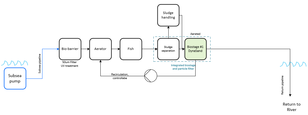
The schematic includes, among other things: subsea pump and intake pipeline; bio-barrier with 50 µm filter and UV; aerator; fish units; sludge separation with separate sludge handling; integrated biostage and particle filter; controllable recirculation pump; return pipeline back to the river. These are the same building blocks as in many modern inland systems, arranged as a clear process chain.
The FlowFarm facility is DABCE's real farming concept - a Swedish "lagom" path toward more sustainable production. The FlowFarm modelling tool, by contrast, is for modelling, comparing and understanding (CAPEX/OPEX, flow, oxygen, treatment) in early stages: feel free to test scenarios, but final design and bankable engineering need more detailed analysis and professional design work.
See also the sections on RAS, raceways, hybrid systems and water quality.
Raceways are long, narrow and relatively shallow culture channels where water flows from one end to the other. They are usually built in concrete, FRP (glass-fibre reinforced plastic) or as earthen channels with liner or other reinforcement. A raceway is primarily a culture unit (tank geometry and hydraulics) - not a production system in the same sense as "flow-through" or "RAS". In practice, raceways most often sit in flow-through, semi-flow-through / partial reuse or hybrid setups where part of the water is treated and returned.
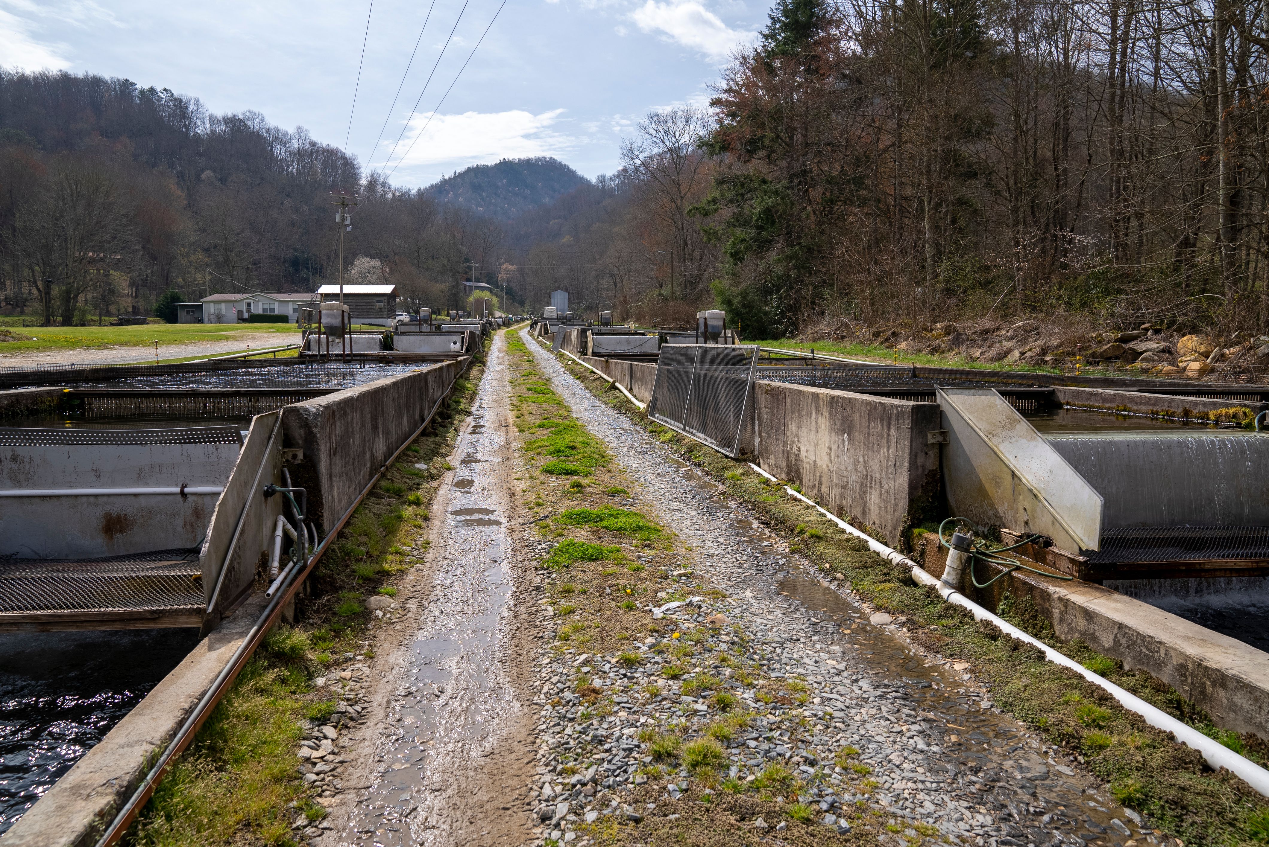
The directed current carries away faeces and feed fines, mixes the water and gives many species a swimming stimulus. Oxygen is partly supplied by the incoming flow, but at higher density and feed load that is rarely enough on its own: modern raceways are often supplemented with pure oxygen (cone, LHO), diffusers or surface aeration. Raceways are among the earliest forms of intensive land-based farming and are still used where there is a stable supply of clean water from springs, rivers, lakes or wells.

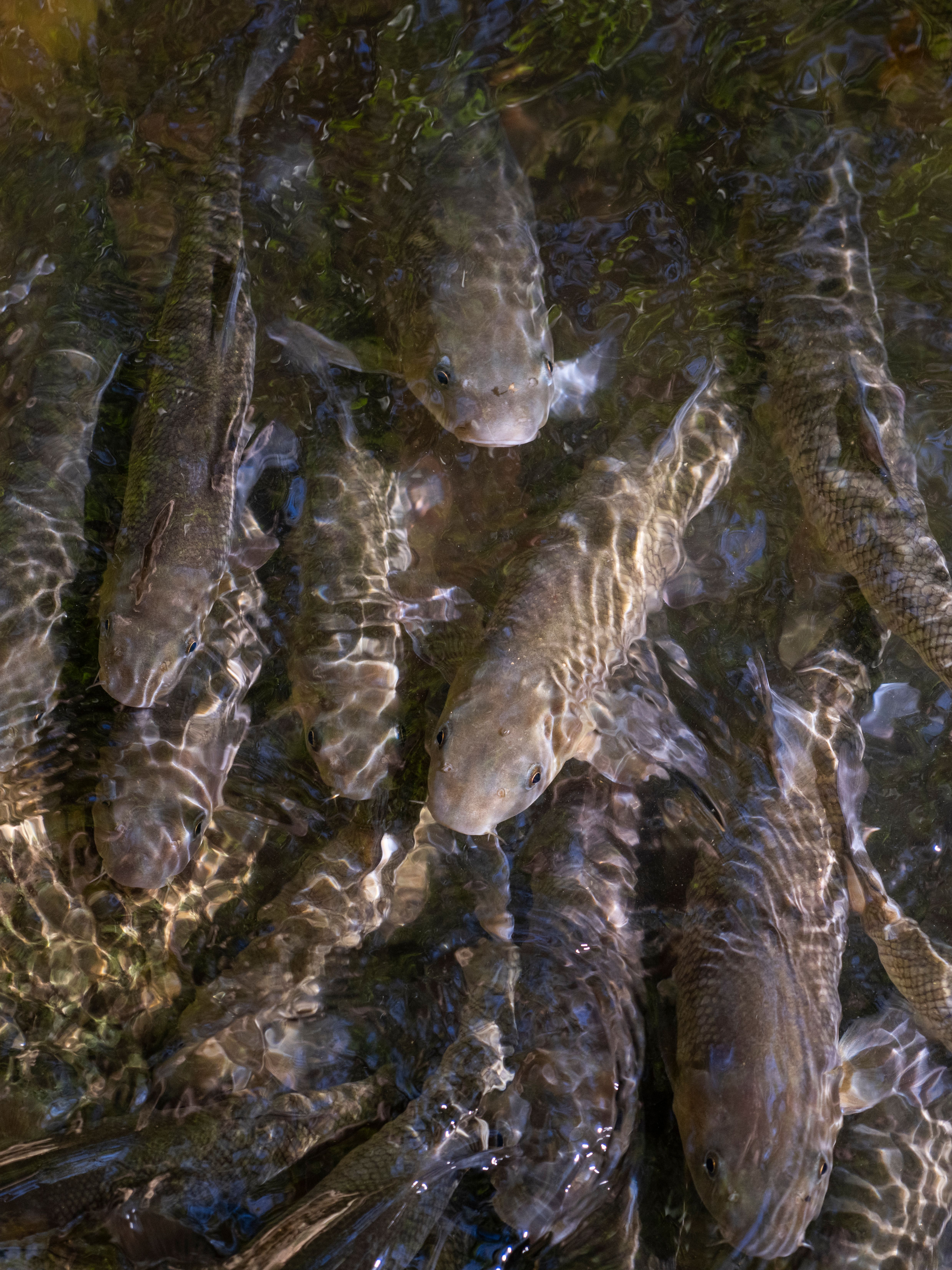
In Europe, classic raceways are mainly linked to cold-water salmonids and related culture: rainbow trout, brown trout, salmon smolt, Arctic char and to some extent whitefish (Coregonus). Sturgeon for meat and caviar is also grown in channels or raceway-like units on some sites. Many Nordic hatcheries and smolt facilities use the raceway principle in parts of the chain - often together with troughs, circular tanks and more closed steps - thanks to simple handling, good overview and proven hydraulics.
Internationally the spectrum is wider. In North America, raceways still dominate much of rainbow trout and hatchery salmonid production. In warmer regions, channels and raceway-like units are used among other things for carp, tilapia and African catfish (Clarias), where the focus is often simple operation, low CAPEX and high volume rather than "natural" current simulation for salmonids.
Some marine and specialty species (e.g. European sea bass, gilthead seabream, eel, barramundi) are sometimes grown in long tanks or channels that resemble raceways, but often with different materials, salinities and flow regimes. Abalone and some other invertebrates have their own raceway-style systems - related in geometry, not the same as a classic freshwater trout raceway. The point is that "raceway" describes a hydraulic form more than a single species list.
Species such as salmon, brown trout, rainbow trout and Arctic char are adapted to flowing water. Raceways mimic parts of that hydraulics: directed flow, swimming stimulus and quick transport of solids toward the outlet. Continuous swimming can support condition and more even growth - provided density, flow and oxygen are sized correctly. For robust species such as carp, catfish and tilapia, the raceway form is more a practical production unit with easy harvest and overview than a "natural river habitat".
Sizing starts from biomass, feed load, species oxygen demand and the water quality you need along the channel - especially dissolved oxygen and solids at the outlet. Pure flow-through is driven mainly by flow; the higher the density, the more critical flow, oxygen addition and solids removal become. Water rights, source quality and receiving-water permits set the outer frame - see also the flow-through section.
Historically, raceways were a central part of early intensive land-based farming, alongside ponds and hatcheries. Today they often act as an intermediate form: the same channel geometry can sit in pure flow-through or be linked to treatment and partial reuse.
Many modern facilities use a chain where raceway volume is combined with process-water treatment:
Raceway (culture unit)
↓
Mechanical filtration
↓
Biofilter
↓
Oxygenation / degassing
↓
Partially returned water
+ make-up from source
(partial reuse / hybrid-RAS)
Such partial-reuse or hybrid solutions keep the handling simplicity of the raceway unit while cutting freshwater need and discharge load versus pure flow-through - without requiring the extreme reuse rate of full RAS.
Raceways can therefore be seen as a historical and practical step between pond culture and more closed systems: full RAS on one side, and semi-flow-through / partial reuse (e.g. DABCE FlowFarm) on the other - where FlowFarm is a buildable semi-flow concept rather than full recirculation.
From an optimisation and engineering perspective, raceways are rarely "the whole answer". They are one piece among several culture units and process steps. A well designed farm often combines different units in a chain where each step matches life stage, risk, cost and site conditions - rather than forcing all production into a single tank form.
Typical building blocks that can be mixed in the same project or value chain:
When several units and life stages sit in the same facility or value chain, flow and biosecurity design become critical. The ideal is to separate water flows between zones - e.g. hatchery/quarantine, juveniles and grow-out - so that a pathogen is not carried "backwards" in the chain via shared return water, common sumps or uncontrolled reuse. Where full hydraulic separation is not practical (shared source, partial reuse, same receiving water), carefully sized bio-barriers are needed at critical points instead: solids removal before disinfection, then e.g. UV and/or ozone (often in series), sometimes with residual-ozone handling, on make-up, transfer water or between zones. A barrier is only as strong as its weakest link - turbid water, wrong UV dose, bypass or shared equipment undermines the effect.
Example chains: hatchery in small tanks → raceway or semi-flow on land → finish in cages; or pond-based start in warmer climates → intensification in channels; or a fully land-based chain with raceways in flow-through where the source is strong, and more closed steps where water or discharge is the bottleneck. Optimal design depends on species, life stage, water supply and temperature, receiving water and permits, energy and labour, market and logistics, and risk profile (disease, escapes, storms, ice).
The point is to assign the right unit to the right step - and to see the farm as an engineering puzzle where raceways, small tanks, ponds, cages and treatment can be combined into a whole that fits the site. There is rarely a universal "best" raceway farm; there are solutions that are proportionate to local conditions.
See also Flow-Through Systems (water rights, receiving water, FlowFarm model), RAS, hybrid systems, ponds, net pens, and the sections on oxygen, solids and biosecurity.
Ponds are one of the oldest and still most important production forms in aquaculture. Despite growing attention on RAS and high-tech land-based systems, a very large share of world aquaculture production still takes place in various pond types - especially in Asia, Africa and Latin America.
From satellite imagery, some regions show vast areas covered by aquaculture ponds. Along coasts and river deltas in e.g. India, Bangladesh, Vietnam, Thailand, Indonesia, China and Ecuador, pond systems sometimes form continuous landscapes over tens or hundreds of square kilometres. In several of these areas, pond culture is among the dominant food industries.
Ponds are built in many ways depending on climate, soil, materials and production goals:
The simplest ponds are embanked land with earthen dikes. In more intensive production, plastic liners are often used to reduce seepage and sediment issues and stabilise water quality. Area per pond can range from a few hundred square metres to several hectares; depth is often about 0.8-2.5 m depending on species, climate and strategy.
Pond culture is used for a very wide group of organisms. In freshwater, common examples include carp (common, grass, silver, bighead), tilapia, pangasius, Clarias catfish, channel catfish, sturgeon, gourami, tambaqui/pacu and regional freshwater species. In brackish and marine water, mullet, milkfish, barramundi and in some cases sea bass/seabream are grown in lagoon- or pond-like units. Shellfish in ponds is globally huge: whiteleg shrimp (Litopenaeus vannamei), black tiger (Penaeus monodon), other penaeids and freshwater prawns (Macrobrachium). Add crabs, sea cucumbers, algae/macroalgae and shallow lagoon culture of mussels/oysters in some systems.
In Europe, ponds are often associated with carp culture, sturgeon for meat/caviar, recreational fisheries and more extensive freshwater farming. In Asia, by contrast, pond culture is the backbone of the aquaculture sector and accounts for enormous volumes of world fish and shellfish production.
When many people think of aquaculture they picture salmon cages or modern RAS. Globally, however, the classic shrimp pond is among the most widespread intensive production forms. A large share of the world's farmed penaeid shrimp is still produced in earthen / mud ponds, especially in India, Vietnam, Thailand, Indonesia, Bangladesh, China and Ecuador. Ponds can be several hectares; whole coastal landscapes in parts of Southeast Asia and Latin America are dominated by shrimp culture.
In extensive ponds, photosynthesis and moderate water exchange can supply enough oxygen. In intensive production, mechanical aeration is almost always used. The most iconic technology is the paddlewheel aerator - floating units with rotating paddles that throw water into the air.
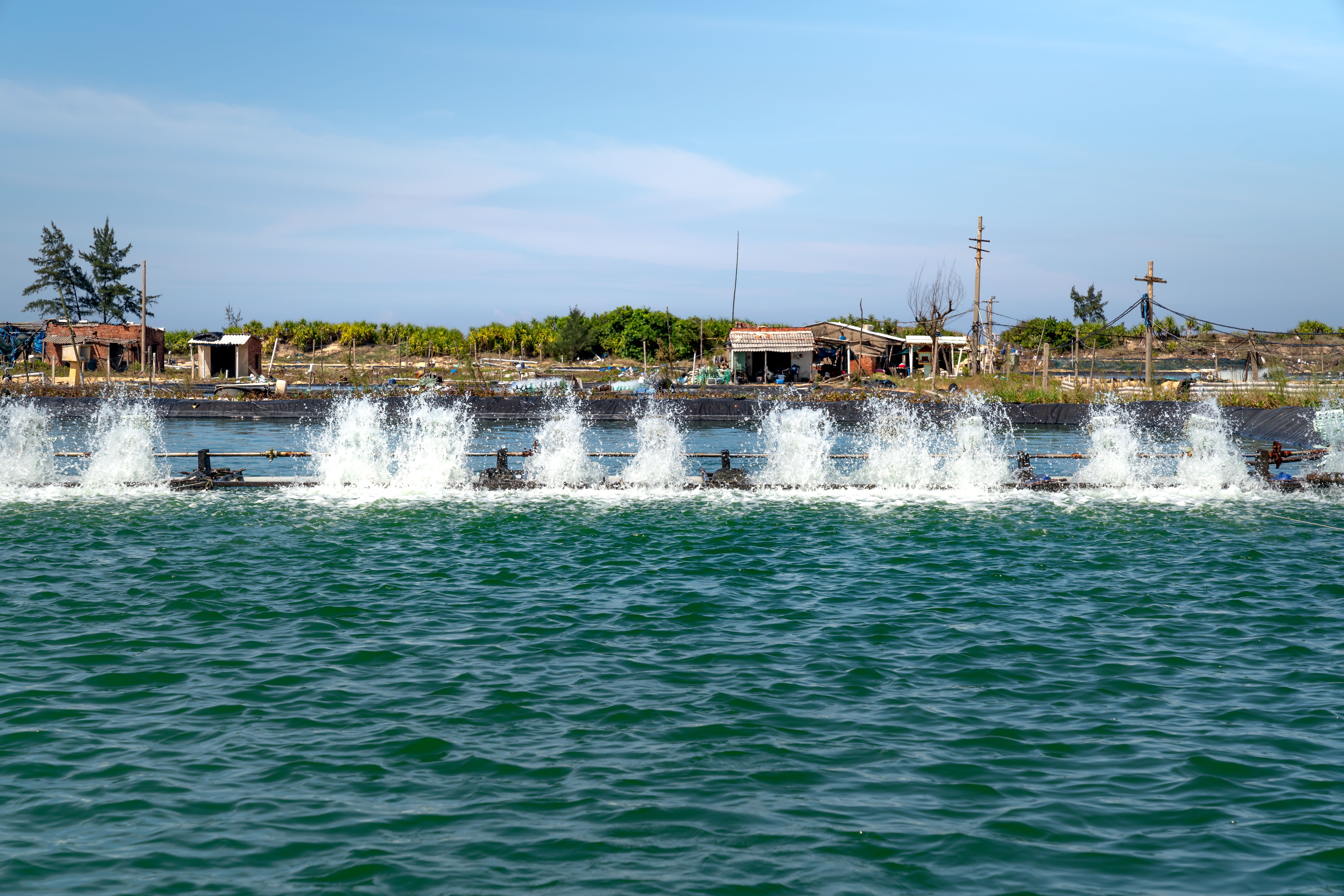
On modern shrimp farms, long rows of paddlewheels may run around the clock during the cycle. Other common techniques: diffusers, aspirators, propeller aerators, fountain aerators, pure oxygen injection, and micro- and nanobubble systems on more advanced sites.
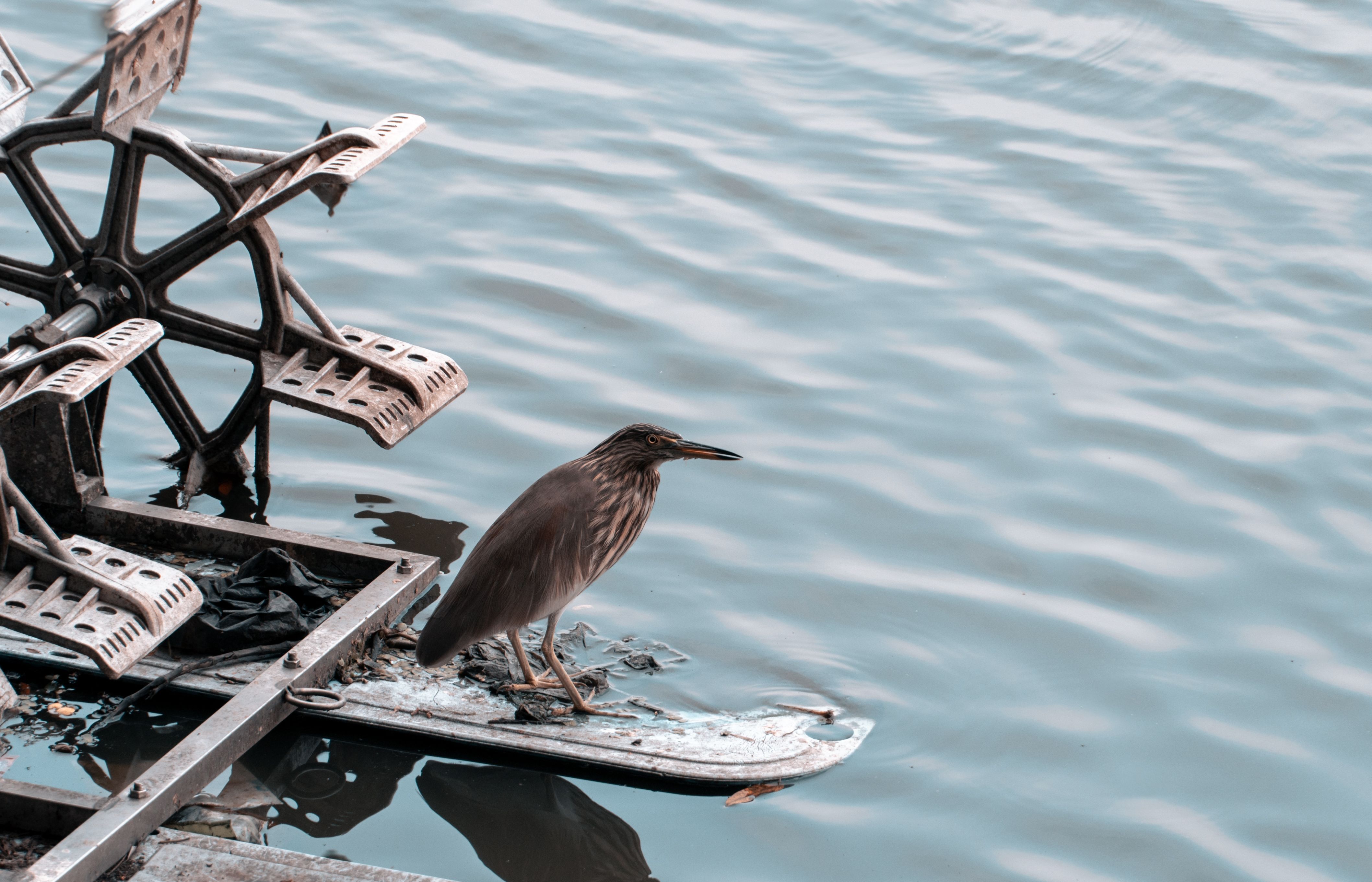
One of pond culture's strengths is that the pond acts as an ecosystem. Besides added feed, it often produces phytoplankton, algae, zooplankton, bacteria, benthos and biofilms. Many species - especially carp, tilapia and shrimp - can use part of that natural production. Pond systems can therefore yield large biomass with relatively low technical complexity, provided nutrient balance, oxygen and sediment are managed.
Where water is scarce or environmental rules tighten, there is a gradual shift toward more controlled solutions: biofloc, partial reuse, hybrid facilities, lined ponds with stronger aeration and in some cases links to land-based treatment. Ponds can also be one step in a production chain - e.g. juveniles in more controlled units then grow-out in ponds, or the reverse - together with raceways, cages and RAS. See also design considerations under Raceways.
At the same time, ponds are likely to remain one of the world's most important production forms for the foreseeable future thanks to simplicity, low cost and the ability to produce large amounts of food where climate and land allow. Advanced concepts such as full RAS and semi-flow (e.g. DABCE FlowFarm) are complements and alternatives where site, species and rules require higher control - not an immediate replacement for global pond volume.
Sources/overview (selection): FAO (production and SOFIA), World Aquaculture Society, Tidwell (ed.) Aquaculture Production Systems (Wiley-Blackwell), Eurofish, NACA, and industry/statistics material on carp, tilapia, shrimp and pond culture. See also land vs sea, raceways, net pens and biosecurity.
Net-pen (cage) farming means fish grow in floating or moored net volumes in the sea, fjord, bay or a freshwater lake. The farmer supplies feed, nets, mooring, monitoring and harvest - but the water is the surroundings: temperature, oxygen, current, ice, algae and pathogens arrive "free" and uncontrolled. This is the model that made Atlantic salmon a global industry, and it remains the backbone of Norwegian, Chilean, Scottish, Faroese and Canadian salmon production.
A typical marine pen is a circular float collar (often HDPE) with a hanging net bag, bottom, weights and sometimes bird or predator nets. Several pens sit in a frame or in rows and are moored to the seabed with chain, rope and anchors. Feed comes from a barge or shore station via hoses; cameras and sensors control the ration. Nets are changed and cleaned; biofouling raises drag and cuts through-flow if it is not managed.
Marine cage farming (salmon, sea bass, sea bream, some tropical species) uses large water volume, salt and often good exchange. The price is lice (on salmon), storms, escapes toward wild stocks, and local benthic load under the pen. Freshwater cages (rainbow trout, Arctic char, sometimes other inland species in the Nordics and elsewhere) avoid sea lice but meet ice, winter oxygen risk, algal blooms and often tighter local lake rules. An inland pen is not "the same farm as in Norway, just in a lake".
Nutrients and solids from feed and faeces enter the water column and the seabed under and around the pen. Modern permits often require environmental monitoring, fallowing, biomass caps and sometimes relocation or technology. Social licence - neighbours, capture fisheries, tourism, wild salmon stocks - is often as decisive as the hardware. The pen is cheap per tonne when it works; it is politically and environmentally sensitive when it does not.
The pen is not the opposite of land-based - they are often coupled. Common: hatchery and smolt/post-smolt on land (higher biosecurity), then on-growing in cages. Conversely, land-based food fish can replace cages where lice, ice, permits or market proximity make open water unsuitable. See land vs sea, offshore, hybrid systems and biosecurity. For inland salmonids where cages are not an option, semi-flow / FlowFarm and RAS are the usual alternatives.
Sources/overview (selection): FAO (production and SOFIA), established marine salmon practice, national lice/discharge rules, and experience from freshwater pens in cold inland waters. Lice limits, biomass and discharge figures are always site- and permit-specific.
Offshore (exposed ocean farming) means sites further out and more open than sheltered fjords and bays: more wave height, more current, greater depth, longer to port. The driver is often the same - more space, less coastal conflict, hope of better water exchange and in some cases lower lice and benthic impact near shore. The price is structure, vessels, weather windows, crewing and insurance in an environment closer to offshore energy than to classic cage farming.
There is no sharp legal line that every country calls "offshore". In practice it is a spectrum: from more exposed coastal sites to truly open ocean. The further out, the more the pen, mooring and logistics must be sized for extreme loads - and the fewer days it is safe to work on the site.
Exposed units are in practice built with the same structural thinking as the rest of the offshore industry. Structural steel - welded jackets, hulls and decks as in oil and gas and marine - is the usual choice: known classing, yard capacity, maintenance and fatigue design against wave and current. Large concrete structures can also be viable, as for some oil platforms and floating concrete hulls: mass, stiffness and corrosion resistance against a heavier formwork and transport job. The choice is not "fish farm vs platform" but load, depth, mooring, service life and which yard or casting site can deliver.
Both routes imply significant CAPEX: classed structure, mooring, offshore installation and spare capacity. OPEX follows the same logic as oil and gas and marine service - not a sheltered coastal pen. Marine supply vessels, weather windows, crew, bunkering, crane lifts, inspection and maintenance at sea are recurring cost items. The further out and the heavier the unit, the more the economics are driven by vessel time and uptime, not only by feed and growth.
Further out, water exchange can be higher and conflict with near-shore use lower. Some concepts aim at larger single units and more automated operation to offset the fewer working days. Offshore is also discussed as a way to move production away from sensitive fjords and wild salmon rivers. It is a direction - not a proven replacement for the coastal pen everywhere.
Alongside "a larger pen further out", more closed floating units are being developed: walls or liners that separate culture water from the surroundings, with pumping, filtration and sometimes lice exclusion. They aim at biosecurity and discharge control but are heavier, costlier and more energy-hungry than an open net bag. They belong in the same family as hybrid and land-based solutions more than classic cages.
Offshore is interesting where the coast is full, conflict is high and capital can fund marine infrastructure. It is rarely the first step for inland salmonids, small projects or sites without a port and service fleet. For Nordic inland sites, land-based semi-flow, raceway or RAS is usually the relevant path - not an exposed ocean pen. See net pens, land vs sea, hybrid systems and FlowFarm.
Offshore is a spectrum of exposure, not a standard product. Structure, insurance and permits are site- and country-specific. This text is orientation - not classing or engineering of an exposed facility.
Most real farms are hybrids - not pure textbook cases. Water is partly reused, juveniles start on land and grow on in cages, or effluent is treated harder than in classic flow-through. Hybrid thinking is often what makes a project permit- and economically possible: enough control where risk is high, simple enough technology where nature already does the work.
Full RAS gives maximum control but high CAPEX, electricity and skill demand. Pure flow-through or an open pen is cheaper but vulnerable to permits, lice, drought and discharge. Hybrid puts treatment and reuse where they pay most: solids and biosecurity early in life, effluent polish toward the receiver, temperature and oxygen buffer when the source fails. It is also how many existing inland salmonid farms evolve - stepwise, not as a jump to a closed loop.
DABCE FlowFarm™ is a buildable semi-flow-through example: intake with protection and filtration/UV, aeration, fish units, sludge separation and an integrated biostage/particle filter with controllable recirculation and return to the receiving water. It sits between pure flow-through and full RAS - more control and lower discharge than a classic raceway, without the heaviest RAS investment. See also flow-through for the process chain and schematic.
Other hybrids (e.g. post-smolt on land + marine cage) solve a different problem: lice and early seawater mortality, not inland water balance. Choose the hybrid for the problem you actually have - not after a generic "more technology is better" rule.
Hybrid is a spectrum. The FlowFarm model is for early comparison (flow, oxygen, treatment, CAPEX/OPEX framing) - not bankable engineering. See RAS, flow-through, net pens and water quality.
Temperature is one of the most important water-quality parameters in aquaculture. It directly influences fish metabolism, appetite, growth rate, oxygen consumption, immunity, digestion, reproduction and overall welfare. Unlike mammals, fish are ectothermic ("cold-blooded"): body temperature closely follows the surrounding water. Even small temperature changes can therefore have significant effects on performance and health.
As water temperature rises, fish metabolism accelerates. Fish eat more, grow faster and become more active, but they also consume more oxygen and produce more waste (ammonia and carbon dioxide). At the same time, warmer water holds less dissolved oxygen. This combination is one of aquaculture's core challenges: oxygen demand increases while oxygen availability decreases.
Temperature therefore influences nearly every part of the farm: growth and feed conversion (FCR), oxygen demand, biofilter performance, ammonia toxicity, disease pressure, energy for heating and cooling, and production planning and harvest timing. See also the sections on dissolved oxygen, carbon dioxide and RAS.
Different species have evolved for different thermal environments. A temperature that produces rapid growth in one species may cause severe stress in another.
Cold-water species - e.g. Arctic char (Salvelinus alpinus), Atlantic salmon (Salmo salar), rainbow trout (Oncorhynchus mykiss) and brown trout (Salmo trutta) - thrive in cool, oxygen-rich water and are often farmed in northern Europe, North America and mountain regions. Warm-water species - e.g. tilapia, carp, catfish, pangasius and kingfish (Seriola lalandi) - often grow best in warmer water (roughly 18-30 °C depending on species) and are farmed in temperate to tropical regions as well as in heated RAS. The same logic applies to shrimp and algae: tropical shrimp and many red seaweeds want warm water, while sugar kelp (Saccharina) is a cold-water species.
| Species | Preferred range (°C) | Growth slows below | Increased risk above |
|---|---|---|---|
| Cold-water fish | |||
| Arctic char | 8–14 | 4–6 | 16–18 |
| Rainbow trout | 10–16 | 6 | 20–22 |
| Atlantic salmon | 8–14 | 4–5 | 18–20 |
| Warm-water fish | |||
| Common carp | 20–28 | 12 | 32–35 |
| Tilapia | 24–30 | 16–18 | 34–36 |
| African catfish | 25–30 | 18 | 34–36 |
| Kingfish / yellowtail (Seriola lalandi) | 18–26 | 15–16 | 28–30 |
| Shrimps | |||
| Whiteleg shrimp (L. vannamei) | 26–30 | 22–24 | 32–35 |
| Black tiger shrimp (P. monodon) | 26–32 | 20–22 | 33–35 |
| Kelp and algae | |||
| Sugar kelp (Saccharina) | 10–15 | 5–8 | 17–20 |
| Tropical red algae (Kappaphycus) | 25–30 | 22–24 | 32–34 |
| Microalgae (typical culture) | 18–28 | 12–15 | 32–35 |
Typical culture windows - exact values depend on genetics, life stage, salinity, dissolved oxygen and husbandry. Algae and shrimp are not fish; ranges are culture windows, not a species protocol.
Temperature ranges by species
 © 2026 DABCE AB
Same typical culture windows as the table. Orientation - not a species protocol.
The relationship between temperature and oxygen is fundamental. Cold water can hold much more dissolved oxygen than warm water. At the same time, fish require more oxygen as temperature rises.
| Water temperature (°C) | Approximate oxygen saturation (mg/L) |
|---|---|
| 0 | 14.6 |
| 5 | 12.8 |
| 10 | 11.3 |
| 15 | 10.1 |
| 20 | 9.1 |
| 25 | 8.3 |
| 30 | 7.6 |
Approximate saturation in freshwater at sea level (1 atm). Salinity, pressure and actual percent saturation change the field value.
A trout farm at 20 °C therefore has roughly 20% less oxygen available than the same farm at 10 °C, while the fish simultaneously need more oxygen. In intensive RAS and flow-through this often becomes the primary production bottleneck. Curves for air and pure O₂ at different pressures are under dissolved oxygen (DO).
Growth generally follows a bell-shaped curve. As temperature increases, growth accelerates until an optimum is reached. Beyond that point feed conversion deteriorates, stress increases and growth declines. Operating outside the optimal thermal range often means reduced feed intake, poorer FCR, slower growth, higher mortality and greater disease susceptibility.
Rainbow trout can grow very well in RAS around about 13 °C, provided oxygen and nutrition are maintained. That is a common target range in controlled salmonid facilities - not a universal recipe. Arctic char generally needs cooler water; tilapia and carp the opposite.
Disease outbreaks often become more likely under thermal stress. Rapid temperature swings can weaken immunity. Many pathogens also reproduce faster at elevated temperatures.
That is why a target value is not enough - stability matters as much as the level itself.
RAS makes it possible to hold a more stable temperature than ponds or cages: year-round growth, more predictable harvest, often better FCR and less seasonal swing. The price is energy. Heating, cooling, pumps, heat exchangers and oxygen must all be designed together with temperature control.
Many modern facilities recover energy via heat exchangers, waste heat, ground-source systems, district heating or heat pumps. In cold inland sites (e.g. Arctic char), summer cooling can be as governing as winter heating. See RAS, heat pumps and chillers under equipment.
Outdoor systems follow nature. Summer: lower oxygen, more algal blooms, higher fish oxygen demand, heat-stress risk. Winter: slower growth, lower feeding, sometimes ice and under-ice oxygen risk in lakes/pens; on land-based sites heating demand may rise. Production planning - especially ponds and cages - often revolves around these swings. See net pens, ponds and dissolved oxygen.
Good temperature management relies on continuous monitoring, not occasional spot checks.
In digital farms, temperature is often a key input to automated feeding, biomass models, oxygen dosing and predictive analytics. See monitoring systems and AI.
Temperature is much more than a number on a sensor. It determines how fast fish grow, how much oxygen they need, how efficiently feed becomes biomass, and how resistant they are to disease. A few degrees can separate exceptional production from severe biological stress - whether farming trout in a Nordic RAS, tilapia in tropical ponds or salmon in net pens. Understanding and controlling temperature is therefore one of the foundations of successful aquaculture.
Sources/overview (selection): FAO Fisheries & Aquaculture; established RAS literature (e.g. Timmons & Ebeling); standard freshwater oxygen-solubility tables. Ranges and saturation figures are indicative - use species, life stage and site data in design.
For farmers, investors or anyone who wants the basics: like people, fish need oxygen to live. The difference is that we breathe air while fish take up oxygen dissolved in water across the gills. If dissolved oxygen falls too low, fish struggle to respire - roughly like a human in a very thin atmosphere.
The air we breathe is roughly 78% nitrogen, 21% oxygen gas and about 1% other gases. When water is aerated with ordinary air, only about one fifth of the gas is actually oxygen. Many modern aquaculture facilities therefore use pure oxygen (100% O₂) instead of air alone. That makes higher density possible and keeps oxygen supply stable even at high feed rates and biomass.
Oxygen drives fish metabolism: swimming, growth, digestion, immunity and reproduction. The more the fish eat and grow, the more oxygen they need.
When oxygen starts to fall you often see increased stress, poorer growth, higher feed conversion ratio (FCR), greater disease susceptibility and fish crowding toward inlets or aeration zones - in the worst case mass mortality. Oxygen is therefore often described as aquaculture's most important water-quality parameter.
Dissolved oxygen (DO) is the concentration of oxygen dissolved in water, usually in mg/L (roughly the same as ppm in water) or as percent saturation. How much oxygen can dissolve at maximum depends mainly on temperature, salinity, air pressure and elevation. Cold water can hold much more oxygen than warm water.
mg/L in freshwater. Air = 20.95% O₂. Pure O₂ at the stated absolute pressure. Gas phase assumed water-saturated.
Air and pure O₂ at 1 atm
Pure O₂ at different absolute pressures
| °C | Air, 1.0 atm | Pure O₂, 1.0 atm abs | Pure O₂, 2.0 atm abs | Pure O₂, 3.0 atm abs | Pure O₂, 5.0 atm abs |
|---|---|---|---|---|---|
| 0 | 14.6 | 69.8 | 140.0 | 210.3 | 350.7 |
| 5 | 12.8 | 61.0 | 122.5 | 184.0 | 307.0 |
| 10 | 11.3 | 53.9 | 108.4 | 163.0 | 272.1 |
| 15 | 10.1 | 48.1 | 97.1 | 146.1 | 244.0 |
| 20 | 9.1 | 43.4 | 87.8 | 132.3 | 221.2 |
| 25 | 8.3 | 39.5 | 80.2 | 120.9 | 202.4 |
| 30 | 7.6 | 36.1 | 73.8 | 111.4 | 186.7 |
Curves: Benson & Krause / Standard Methods air saturation at 1 atm, scaled by Henry's law (O₂ mole fraction and (P − pH₂O)). Theoretical equilibrium - not transfer efficiency in a cone/LHO. Actual tank DO is lower because of transfer losses, consumption and the culture volume being open to 1 atm. 2–5 atm abs is a typical cone/LHO pressure band, not a target in the pen.
For many people outside water chemistry it is surprising that water in equilibrium with air only holds about 7-13 mg/L oxygen depending on temperature. That is because air is only about 21% oxygen gas; nitrogen does not supply the fish. With pure oxygen the partial pressure of O₂ rises about fivefold, so much more oxygen can dissolve. If oxygen is added under pressure (e.g. oxygen cone or LHO at about 5 bar absolute), theoretical solubility rises further - so inlet water can be produced well above ordinary air saturation. That is a main reason modern intensive culture often uses pure oxygen systems beyond or instead of aeration alone.
But more dissolved oxygen is not always better. When water is saturated (or supersaturated) under pressure in pipes and oxygen units and then released into culture tanks that are open to the air at about 1 atm, a "soda-bottle effect" can appear: gas wants to leave solution as pressure drops. The result can be bubbles, foam, local supersaturation and uneven gas balance right at the inlet and in jets. Excessively high dissolved oxygen and/or sudden pressure relief can stress fish - including gill irritation, behaviour changes and in serious cases gas bubble disease (especially when total gas pressure and nitrogen are also high). So it is not enough to "max out" DO in the pipe; you must understand how water spreads in the tank - inlet direction, velocity and mixing, dead zones vs short-circuiting, and where the fish actually live. Good hydraulics and controlled inlet mixing distribute oxygen evenly and avoid both local hypoxia and harmful gas pockets. Measure DO where it matters (in the tank, not only in the pressurised line), and see also the section on saturation, supersaturation and N₂.
Without reliable measurement, the oxygen strategy is guesswork. In practice three paths dominate: handheld checks (routine, troubleshooting, calibration control), fixed process sensors linked to PLC/SCADA (continuous trend, oxygen/aeration control and alarms), and sometimes portable loggers or temporary points at commissioning and performance tests. Match technology to risk and density: ponds and low intensity may manage with spot checks; raceways, semi-flow and RAS at high biomass usually need continuous DO where the fish live - often with redundancy on critical units.
Two main types of oxygen sensor are used on farms:
Both types usually show mg/L and % saturation, if temperature (and sometimes salinity) is compensated correctly. Check two things: that the sensor has proper temperature compensation, and that % sat is calculated against the right reference - fresh or salt water, plus elevation/air pressure.
Capacity and performance often specified: a range covering both low DO (emergency) and supersaturation at oxygenated inlets (e.g. 0-20+ mg/L or 0-200% sat depending on model), response time suitable for process alarms (seconds to tens of seconds - not minutes if oxygen drives automation), stability in flowing, particle-laden water, and outputs that fit the plant (4-20 mA, Modbus, digital alarms). Placement is as important as sensor type: avoid dead corners, avoid sitting straight in a pure oxygen jet if you want a tank average, and avoid sucking in air bubbles. For oxygen dosing control one often measures both "critical low" in the tank and sometimes inlet after the oxygen unit - knowing that pipe and tank do not share the same DO.
Problems with oxygen probes (regardless of principle) are common and underestimated: fouling by biofilm, feed oils and particles that make readings sluggish or falsely low/high; drying out or damaged membrane/optical face; wrong or forgotten calibration; temperature errors that hit both mg/L and % sat; cable faults and moisture in connectors; air bubbles or stagnant pockets at the sensor; and "zombie values" that look stable in SCADA while the real tank has already dropped. Probes age and drift - compare regularly against a freshly calibrated handheld reference, keep a spare sensor or probe, and treat alarm limits with common sense (fish behaviour, feed response). Good oxygen measurement is maintenance and placement as much as hardware choice. See also monitoring systems and sensors under equipment / AI & monitoring.
In biological systems oxygen is consumed mainly by fish respiration, biofilters (nitrification), other microbes and breakdown of organic matter. In a RAS, a substantial share of oxygen use can occur in the biofilter rather than in the fish themselves. Nitrification NH₄⁺ → NO₂⁻ → NO₃⁻ consumes large amounts of oxygen and must be included in the oxygen balance.
There is also a biological paradox: warmer water holds less oxygen, while fish need more oxygen as temperature rises. That makes summer operation and high feed rates the most critical periods on many farms.
On a commercial farm, oxygen is in practice a mass-balance question. Every kilogram of feed drives fish respiration, biofilter nitrification and oxidation of organics. Oxygen demand can therefore often be estimated from daily feed - but it is not the average that sizes the system. It is the peak load: peak feed.
Peak feed sizes oxygen tanks, LOX, oxygen cones, LHOs, degassers, emergency power, pumps and emergency systems. Always size oxygen and related hydraulics for maximum daily feed (plus safety margin), not for average seasonal operation.
Feed is the dominant mass input on an intensive farm. The fish convert part of the carbon, nitrogen, phosphorus and energy into growth; the rest leaves as respiratory gases, urine/gill excretion, faeces and feed waste. For salmonids (here exemplified with Atlantic salmon / salmonids in grow-out on modern dry feed), process design can therefore be tied to daily feed in kg/day - but the figures are order-of-magnitude for teaching and early sizing, not bankable design. Feed recipe (protein, fat, digestibility), FCR, temperature, size and waste change the profile strongly.
Simplified biology/chemistry: organic carbon in feed is oxidised to CO₂ (respiration) or leaves as particulate organics (faeces/waste); protein nitrogen not built into biomass is excreted mainly as ammonia/ammonium (TAN) across the gills; phosphorus largely follows faeces and dissolved P; solids load filters and the receiving water. In RAS, TAN is also nitrified in the biofilter (extra O₂ demand and alkalinity use) and solids must be removed before they break down into more dissolved COD/BOD.
Approximate design rules of thumb for 1 kg dry feed to Atlantic salmon/salmonids in good growth (illustrative ranges from established RAS/water-quality practice). Always use feed analysis, measured FCR and site data in hard engineering.
From 1 kg feed — simplified mass-flow picture
Teaching sketch in the spirit of older Swedish EPA (Naturvårdsverket) nutrient-flow figures for fish farms. Not a permit calculation — use feed analysis, measured FCR and current guidance in licensing.
© 2026 DABCE AB
| Parameter (per kg feed) | Typical range | Comment |
|---|---|---|
| O₂ - fish respiration | ~200-300 g O₂ | Often ~0.25 kg O₂/kg feed as a starting value |
| O₂ - nitrification (if all TAN is nitrified) | ~140-200 g O₂ | Stoichiometry ~4.57 g O₂ per g TAN |
| O₂ - total system (fish + biofilter + margin) | ~0.4-0.7 kg O₂ | Size for peak feed + safety |
| CO₂ - respiration (fish etc.) | ~250-400 g CO₂ | Same peak as oxygen; see CO₂ section |
| TAN (total ammonia nitrogen) | ~25-45 g TAN-N | Rises with protein share and poorer retention |
| TSS / solids (faeces + waste) | ~200-400 g | Strongly depends on FCR, pellet and husbandry |
| Phosphorus (P, dissolved + particulate) | ~5-15 g P | Feed recipe and digestibility dominate |
| Organic load (BOD/COD direction) | High - tied to TSS and fines | Drives oxygen need if solids are not removed |
Teaching approximations for salmonids. Not a substitute for mass balance against actual feed and life stage.
Oxygen demand per kg feed (salmonids, approximate mid-range)
Only the O₂ rows in the table can share a pie (same unit). Fish 200–300 g, nitrification 140–200 g; other/margin fills toward about 0.55 kg total (0.4–0.7 kg range). Not a mass balance for CO₂, TAN, TSS or P.
Example (worked illustration, not a fixed answer): peak feed 1,000 kg/day × 0.25 kg O₂/kg feed ≈ 250 kg O₂/day for fish metabolism alone. Add nitrification (e.g. 35 g TAN/kg feed × 4.57 ≈ 160 g O₂/kg feed → ~160 kg O₂/day) and system demand quickly sits around 400+ kg O₂/day before efficiency, losses and safety margin - which is why LOX/PSA, cones/LHO and peak-feed thinking are central in commercial salmonid RAS.
Per kg feed in, one can think of a complete "emission and residue profile" that the farm must handle - either in water treatment (RAS/semi-flow) or via the receiving water (flow-through/cages) within permit limits:
1 kg feed in
↓
Growth (depends on FCR)
+
O₂ consumed (fish + biofilter)
+
CO₂ out (respiration)
+
TAN → (NO₂⁻) → NO₃⁻
+
TSS / sludge (faeces + waste)
+
P and nutrients
+
Heat / residual organics
The design point: do not only count "how much oxygen". Count the whole chain - oxygen, CO₂ stripping, solids, nitrogen and sludge - against the same peak feed. See also carbon dioxide (CO₂), ammonia, sludge handling, FCR and FlowFarm for concept sizing.
One of the most important design parameters is the difference between oxygen into and out of the fish unit. Example: inlet 10 mg/L, outlet 7 mg/L gives ΔDO = 3 mg/L. Larger allowed ΔDO → less water flow needed; smaller ΔDO → more flow. That directly affects pump size, energy use, pipe sizes, tank hydraulics and CAPEX. In many modern RAS facilities, optimising ΔDO (together with oxygen transfer and CO₂ stripping) is among the main levers to cut energy cost.
Pure oxygen is often used at high biomass because transfer efficiency is much higher than with ordinary air - see also the sections on oxygen cones, LHO, aeration and oxygen demand under equipment and oxygen & gas.
Oxygen can never be viewed in isolation. Intensive systems must also manage oxygen supply, carbon dioxide stripping, alkalinity, pH, ammonia load and hydraulics. Many high-intensity facilities are limited by carbon dioxide long before they are limited by oxygen supply. A farm can show good DO values while fish performance is limited by elevated CO₂. See the carbon dioxide (CO₂) section.
Oxygen is in practice the fish farm's equivalent of fuel in an engine. Without enough oxygen, neither the fish, the biofilter nor the production system works as intended. For many modern facilities, oxygenation is therefore one of the most important technical, biological and economic design parameters.
Sources/overview (selection): Boyd & Tucker, Pond Aquaculture Water Quality Management; Timmons & Ebeling, Recirculating Aquaculture; Colt, water quality for aquaculture; Henry's law and standard oxygen solubility tables; established practice for sizing RAS, oxygen cones and LHOs; feed-based mass balances for salmonids (O₂, CO₂, TAN, TSS). Table and feed values are approximate teaching figures - use feed analysis, FCR and site data in engineering design.
For farmers, designers or anyone understanding intensive systems: carbon dioxide (CO₂) forms when fish and microbes respire - roughly the mirror image of oxygen use. Fish take up O₂ and release CO₂ into the water. In open ponds and cages, CO₂ is often diluted by large water volumes and gas exchange with air. In RAS, semi-flow and other high-density, low-exchange systems, dissolved CO₂ can rise until it limits growth and welfare - sometimes while oxygen still looks "fine" on the display.
That is why CO₂ is one of the parameters that separate "enough oxygen" from "fish that actually perform". Modern intensive culture must design for both oxygen supply and carbon dioxide stripping - see also the dissolved oxygen (DO) section.
Dissolved CO₂ affects blood and respiration. High levels lower blood pH (respiratory acidosis), make it harder to load and unload oxygen via haemoglobin systems, and cause stress even when DO in mg/L looks acceptable. Fish may increase ventilation rate, reduce feed intake, lose growth and become more disease-prone. At strongly elevated CO₂ you see lethargy, crowding at the surface or inlet, and in the worst case mortality - often combined with other stressors (heat, low alkalinity, handling).
Tolerance depends on species, life stage, acclimation and how fast CO₂ rises. Salmonids in intensive land-based culture are often held to fairly low targets in literature and practice (many farms aim on the order of single-digit to low tens of mg/L free CO₂ depending on species and policy) - exact limits should be set with species knowledge and veterinary/production standards, not web rules of thumb alone.
In water, CO₂ is part of the carbonate system: dissolved CO₂ (roughly H₂CO₃*) ↔ HCO₃⁻ ↔ CO₃²⁻. When more CO₂ dissolves, the equilibrium shifts, pH falls and the fraction of "free CO₂" rises. Alkalinity (buffer, often measured as HCO₃⁻ equivalents) dampens pH swings: at low alkalinity the same CO₂ addition causes a larger pH drop and more stress. So CO₂, pH and alkalinity belong together - see also the pH and alkalinity sections. In freshwater RAS, bicarbonate/lime make-up may be needed both for the biofilter and to hold buffer when CO₂ is stripped and nitrification consumes alkalinity.
Important: pH alone is not the same as CO₂. The same pH can mean different free CO₂ depending on alkalinity and temperature. So it is rarely enough to "control on pH" if you want to know whether fish are breathing in a CO₂-loaded environment - you need either measured/calculated free CO₂ or a calibrated model against alkalinity and pH.
As with oxygen, peak feed is the sizing load: more feed → more O₂ demand and more CO₂ production at roughly the same time. Summer operation (warmer water, higher metabolism) is often critical for both gases. For salmonids, early design often uses roughly 250-400 g CO₂ per kg feed as an order of magnitude (same uncertainty as for O₂) - see mass balance and emission profile under dissolved oxygen (DO).
Pure oxygen and cones/LHOs can raise inlet DO quickly. Removing CO₂, by contrast, needs gas exchange against a gas phase with low CO₂ partial pressure - typically air in a degasser, cascade or packed column - plus enough contact time and area. If you only "pump in oxygen" without stripping CO₂, you can create a farm with high DO and still reduced feed intake and growth. Many high-intensity systems are therefore CO₂-limited: degasser size, air flow, head and hydraulics set the ceiling, not oxygen gas flow alone.
Best practice in many RAS designs: maximise air-side gas exchange in the degasser (CO₂ out, O₂ in from air), then add pure oxygen to reach the desired total ΔDO - do not replace all aeration with pressurised O₂ alone. That often cuts energy need and the risk of forgetting CO₂. See degassers, LHO, oxygen cones and oxygen demand under equipment and oxygen & gas.
CO₂ is harder to "just put a probe on" than temperature. Common paths: (1) calculate free CO₂ from pH, alkalinity, temperature and salinity with carbonate equilibria - needs reliable alkalinity and pH measurement; (2) direct CO₂ sensors / membrane or NDIR solutions in process water where available and maintained; (3) lab or field kits as spot checks. Online pH is often used as a fast indicator, but as noted above pH is not identical to CO₂ without known buffer.
Practical problems: wrong alkalinity → wrong calculated CO₂; pH electrodes that drift or foul; slow response; measurement in a sump that does not represent the tank; and staff trusting DO alarms while CO₂ quietly rises at peak feed. On high-intensity farms, CO₂ (measured or calculated) should be part of the operating picture together with DO, pH and feed - see monitoring systems.
In short: oxygen is the fuel, but CO₂ is the exhaust. An engine that only gets fuel without an exhaust outlet runs poorly - the same logic applies to intensive fish farming. Good gas balance is O₂ in, CO₂ out, stable buffer and hydraulics that mix the tank evenly.
Sources/overview (selection): Timmons & Ebeling, Recirculating Aquaculture; Boyd & Tucker, Pond Aquaculture Water Quality Management; Colt et al. on gases and water quality; established RAS practice for degassing and the carbonate system. Free CO₂ targets are species- and site-specific - use site data and applicable welfare/production requirements in design.
pH is one of the most important water-quality parameters in aquaculture. It influences fish physiology, oxygen transport, ammonia toxicity, biofilter performance, nutrient availability and overall system stability. Even when oxygen, temperature and filtration look acceptable, poor pH control can cut growth and raise stress.
pH measures how acidic or alkaline the water is on a scale from 0 to 14: 7 is neutral, below 7 acidic, above 7 alkaline. The scale is logarithmic - a change from 7 to 6 is a tenfold increase in acidity. Small pH steps are therefore large chemical changes.
Fish continuously exchange ions and gases across the gills. Water that is too acidic or too alkaline can damage gill tissue, disrupt osmoregulation, raise stress and reduce growth. Sudden swings are usually worse than a slow move. In many cases stability matters more than a precise target.
| pH range | General effect |
|---|---|
| < 5.5 | Dangerous for most cultured fish |
| 5.5–6.5 | Significant stress for many species |
| 6.5–7.5 | Good range for many freshwater systems |
| 7.0–8.0 | Common target range in RAS |
| 8.0–8.5 | Generally acceptable |
| > 8.5 | Increased ammonia toxicity |
| > 9.0 | Potentially harmful |
| > 10 | Dangerous for most fish species |
Freshwater orientation. Most freshwater farms run best around pH 6.8–8.0. Do not apply this table unchanged to brackish or seawater.
Brackish water and seawater have a different background chemistry. Open sea is often around pH 7.8–8.3 (typically near 8.0–8.2) with higher alkalinity than most fresh waters. Brackish water sits in between and follows the mix of fresh and salt, algal production and CO₂. Marine and brackish RAS can still be pulled down by fish CO₂ - then gas control, not "an acidic source", is usually the fix. At pH 8+ the toxic NH₃ fraction is already higher than in near-neutral freshwater: the same TAN is more serious. See salinity, carbon dioxide and ammonia.
| pH range | Brackish / seawater - general effect |
|---|---|
| < 7.2 | Unusual in open sea; in marine RAS often a sign of high CO₂ or spent buffer - stress and weaker nitrification |
| 7.2–7.6 | Low for natural seawater; can occur in closed marine/brackish RAS under CO₂ load |
| 7.6–8.0 | Acceptable in many brackish and marine systems; a common target when CO₂ is controlled |
| 8.0–8.3 | Typical open sea and many net pens / marine RAS in balance |
| 8.3–8.5 | Upper natural seawater; higher NH₃ fraction - keep TAN low |
| > 8.5 | Elevated ammonia risk even at moderate TAN; check algae, degassing and TAN |
| > 9.0 | Potentially harmful - same warning as in freshwater |
Orientation. Natural seawater is more strongly buffered than most fresh waters, but closed marine RAS can still lose pH via CO₂ and nitrification. Species and salinity set the target.
Cold-water salmonids (rainbow trout, Arctic char, Atlantic salmon) often do well around pH 6.8–7.8. Warm-water species such as tilapia, carp, catfish and pangasius often tolerate 6.5–8.5. Tilapia are among the more pH-tolerant farmed fish. Kingfish (Seriola) is usually farmed in more marine or brackish water where background pH is often higher than in freshwater - steer to species and salinity, not a freshwater target.
In RAS, pH is tightly linked to nitrification. Bacteria convert ammonia (NH₃/NH₄⁺) → nitrite (NO₂⁻) → nitrate (NO₃⁻). The process generates acid and consumes alkalinity. Without enough buffer, pH falls over time, nitrification slows or stops, and the system becomes unstable. Alkalinity often has to be topped up - see alkalinity and ammonia.
Total ammonia nitrogen (TAN) exists as NH₄⁺ (ammonium, relatively harmless) and NH₃ (unionised ammonia, highly toxic). As pH rises, a larger fraction becomes NH₃. The same TAN level can be relatively safe at pH 7.0 and dangerous at pH 8.5. Temperature also shifts the equilibrium - always read pH, temperature and TAN together. Calculate the NH₃ fraction in the ammonia section.
In ponds, raceways and algae-rich systems, pH often changes through the day. In the morning photosynthesis is low, CO₂ has built up overnight and pH is typically lowest. In the afternoon algae consume CO₂, pH rises and oxygen often peaks. Large daily swings (sometimes more than one full pH unit in productive ponds) can stress fish even when average pH looks fine. See ponds and dissolved oxygen.
pH and CO₂ are tightly linked. Dissolved CO₂ forms carbonic acid (CO₂ + H₂O ⇌ H₂CO₃) and lowers pH. When CO₂ is stripped (degassing, aeration or photosynthesis), carbonic acid falls and pH rises. In intensive RAS many "pH problems" are actually poor CO₂ control. See carbon dioxide (CO₂).
Alkalinity is the water's ability to neutralize acid and resist a pH drop. In aquaculture it is mainly the carbonate system: bicarbonate (HCO₃⁻), carbonate (CO₃²⁻) and dissolved CO₂. pH shows the condition now; alkalinity shows how much buffer remains. Simplified: CO₂ ⇌ H₂CO₃ ⇌ HCO₃⁻ ⇌ CO₃²⁻. When acid is added, bicarbonate/carbonate take up H⁺ and pH falls more slowly.
In RAS, nitrification consumes alkalinity continuously. Without make-up, pH falls, the biofilter loses performance and a pH crash can come suddenly when the buffer is gone. Two farms at the same pH can therefore behave very differently - one is stable, the other close to collapse. Treat alkalinity as a consumable, much like oxygen. See alkalinity.
| Alkalinity (as CaCO₃) | Interpretation |
|---|---|
| < 50 mg/L | Low buffering capacity |
| 50–100 mg/L | Moderate buffering |
| 100–200 mg/L | Common operational target |
| 200–300 mg/L | Strong buffering |
| > 300 mg/L | Very high buffering capacity |
Typical freshwater/RAS bands. Targets depend on species, feed load, nitrification, source and strategy.
Common ways to hold alkalinity: sodium bicarbonate (NaHCO₃), calcium carbonate (limestone), dolomite, calcium hydroxide, sodium carbonate. Sodium bicarbonate is widely used in commercial RAS - it replenishes HCO₃⁻ and is relatively easy to handle. Degassing removes CO₂ and often raises pH; more bicarbonate mainly strengthens resistance to future pH decline, not necessarily a dramatic pH jump.
Reduced feeding, flashing/rubbing, increased gill movement, surface aggregation, erratic swimming, poor growth and more disease. The same picture can be oxygen, ammonia or CO₂ - measure, do not guess. See monitoring systems.
Temperature determines how fast biology works. Oxygen determines whether fish can breathe. pH determines whether water chemistry stays stable enough for everything else to function. Alkalinity tells you how resistant the system is to becoming acidic tomorrow.
Sources/overview (selection): Timmons & Ebeling, Recirculating Aquaculture; Boyd & Tucker, Pond Aquaculture Water Quality Management; established RAS practice on the carbonate system, nitrification and ammonia equilibrium. Ranges are indicative - use species, salinity and site data.
Alkalinity is one of the most important but often overlooked water-quality parameters in aquaculture. pH says how acidic or alkaline the water is right now. Alkalinity says how much the water can take before pH collapses.
In most freshwater farms the buffer is the carbonate system: CO₂ ⇌ H₂CO₃ ⇌ HCO₃⁻ ⇌ CO₃²⁻. Bicarbonate and carbonate take up hydrogen ions (H⁺) from biology and slow a pH drop.
A simple rule: pH shows where chemistry stands today. Alkalinity shows how resistant the system is to becoming more acidic tomorrow. See pH and carbon dioxide (CO₂).
Alkalinity supports both fish health and the biofilter. In RAS, nitrifiers continuously convert ammonia (NH₃/NH₄⁺) → nitrite (NO₂⁻) → nitrate (NO₃⁻). The process releases H⁺ and therefore consumes alkalinity. Without enough buffer, pH becomes unstable, nitrification slows, feed capacity may be limited, and a sudden pH crash becomes possible. Treat alkalinity as a consumable — much like oxygen. See Ammonia / TAN and dissolved oxygen.
With enough alkalinity, pH changes slowly, nitrifiers work steadily and TAN removal stays predictable. When the buffer is gone, small acid additions can swing pH a lot, the biofilter can drop off and nitrite can rise. Two farms at the same pH can therefore behave very differently: strong buffer is stable; low alkalinity may be days from a crash.
| Alkalinity (as CaCO₃) | Interpretation |
|---|---|
| < 50 mg/L | Low buffering capacity |
| 50–100 mg/L | Moderate buffering |
| 100–200 mg/L | Common operational target |
| 200–300 mg/L | Strong buffering |
| > 300 mg/L | Very high buffering capacity |
Typical freshwater/RAS bands. Targets depend on species, feed load, source, density and biofilter loading.
Read the three together. More CO₂ lowers pH. Degassing removes CO₂ and usually raises pH. Adding alkalinity increases buffer capacity — it does not always raise pH dramatically, but it makes future pH drops less likely. Many "pH problems" in intensive culture are actually too little alkalinity or poor CO₂ control.
Freshwater RAS often needs continual top-up to replace what nitrification consumes. Common additions: sodium bicarbonate (NaHCO₃), calcium carbonate (limestone), dolomite, calcium hydroxide, sodium carbonate. Sodium bicarbonate is common in commercial RAS — it replenishes HCO₃⁻ and is relatively easy to dose. No dose here: calculate against feed load and measure.
Alkalinity is usually reported as mg/L CaCO₃ (calcium carbonate equivalent), sometimes meq/L. It changes more slowly than DO or pH, so daily measurement is often unnecessary — but regular checks are good practice in intensive farming. Especially when raising feed load, expanding biomass, starting a biofilter, seeing unexplained pH drops, or adjusting bicarbonate dose.
pH tells you how the water behaves today. Alkalinity tells you how resilient the system will be tomorrow. A stable pH with low alkalinity may mean a crash is approaching. Strong buffer helps keep biofilter performance, fish health and water chemistry predictable through the cycle.
Sources/overview (selection): Timmons & Ebeling, Recirculating Aquaculture; Boyd & Tucker, Pond Aquaculture Water Quality Management; established RAS practice on the carbonate system and nitrification. Ranges are orientation, not permit values.
Hardness is a measure of dissolved divalent minerals in water, mainly calcium (Ca²⁺) and magnesium (Mg²⁺). They matter for osmoregulation, skeleton, reproduction and stable water chemistry. Hardness and alkalinity are both often reported as mg/L CaCO₃ — but they measure different things. Hardness is mineral content. Alkalinity is the ability to resist acidification. See alkalinity.
Fish are in constant contact with the water and exchange ions across gills, skin and gut. Dissolved minerals are therefore not only "chemistry on paper" — they are part of the fish's internal balance.
Very soft water forces the fish to spend more energy on salt balance. That can cut growth, raise disease sensitivity and hurt reproduction. Hardness can be raised by mineralisation treatment: let the water trickle over a bed of crushed limestone or similar (example from another industry: common on ships, where evaporator or RO water is almost mineral-free and must be post-treated before use).
Hardness comes mainly from Ca²⁺ and Mg²⁺. Alkalinity comes mainly from HCO₃⁻ and CO₃²⁻. A source can therefore have high hardness and low alkalinity — or the reverse — or high or low values of both. Both matter, for different reasons.
Calcium supports egg membranes, fertilisation, water regulation in the egg, the embryo and hatching. Extremely soft water can mean poorer hatch, fragile eggs, more deformities and weak larvae. Many hatcheries therefore watch hardness, calcium, alkalinity and conductivity as closely as oxygen and temperature.
| Ion | Main role |
|---|---|
| Calcium (Ca²⁺) | Bone, gills, egg quality |
| Magnesium (Mg²⁺) | Enzyme activity, metabolism |
| Sodium (Na⁺) | Osmoregulation |
| Potassium (K⁺) | Nerve and muscle |
| Chloride (Cl⁻) | Osmoregulation, nitrite protection |
| Bicarbonate (HCO₃⁻) | Buffering / alkalinity |
| Sulphate (SO₄²⁻) | Natural water chemistry |
| Trace elements | Various biological functions |
Two sources with the same hardness can behave differently if the ion mix differs. Advanced hatcheries and RAS often measure conductivity and individual ions, not only total hardness.
In groundwater, Fe²⁺ and Mn²⁺ are often more important in practice than hardness itself. When the water meets oxygen the metals oxidise and precipitate: Fe²⁺ → Fe³⁺ → Fe(OH)₃ and Mn²⁺ → MnO₂(s). The particles can irritate gills, foul drum filters, biofilters, nozzles and sensors, and increase sludge.
Common pretreatment: aeration, degassing/cascade, sand filters, oxidation and catalytic media. Fe and Mn technically count toward hardness as divalent ions, but on a farm the issue is mostly fish health and fouling. For many groundwater sites, Fe/Mn is a bigger job than hardness. See also filtration and aeration under equipment.
| Hardness (mg/L as CaCO₃) | Classification |
|---|---|
| 0–60 | Soft water |
| 60–120 | Moderately hard |
| 120–180 | Hard water |
| > 180 | Very hard water |
Many freshwater farms run well around 50–250 mg/L CaCO₃. The ideal depends on species, life stage and strategy. Orientation, not a protocol.
Put hardness and alkalinity on the same plot and a rough target region appears for most freshwater farms. The box is orientation, not a requirement — and it does not replace species- or source-specific analysis.
Green box: hardness about 50–250 mg/L and alkalinity about 80–200 mg/L (as CaCO₃). Orientation — species, life stage and source govern. Not a permit value.
© 2026 DABCE AB
Adequate calcium can reduce sensitivity to nitrite, aluminium, some metals and other stress. Fish in soft water are often more sensitive to disturbances than fish in harder water. See nitrite.
In RAS, mineral content can drift with water exchange, solids removal, source chemistry, treatment and biology. Rainwater, RO water and very soft groundwater may need remineralisation. Low hardness can mean poorer hatchery results, poorer welfare, a less stable biofilter and more physiological stress.
Common additions: calcium carbonate (limestone), dolomite, calcium chloride, magnesium sulphate (Epsom salt) and commercial blends. The aim is rarely "as hard as possible" but enough minerals and stable operation. No dose here — calculate against analysis and species.
Total hardness (TH) as mg/L CaCO₃, by kit, lab or online. In hatcheries and advanced RAS it is often worth measuring Ca, Mg, Fe, Mn, conductivity and alkalinity separately.
Alkalinity stabilises the chemistry. Hardness provides the minerals. Iron and manganese decide how much pretreatment a groundwater source may need before it is fit for aquaculture. For osmoregulation, individual ions and conductivity, see mineral and ion management.
Sources/overview (selection): Timmons & Ebeling, Recirculating Aquaculture; Boyd & Tucker; established hatchery and RAS practice. Ranges are orientation, not permit values.
Fish do not simply live in water. They live in a complex chemical environment containing dissolved gases, minerals, nutrients, salts, and organic compounds. Every second, water passes across the gills where fish absorb oxygen, release carbon dioxide, excrete ammonia, and continuously exchange ions with their surroundings.
The most important dissolved ions include:
Together, these ions influence nearly every aspect of fish biology, including respiration, growth, stress tolerance, reproduction, immunity, and energy use.
Unlike terrestrial animals, fish are constantly exposed to the water around them. Their internal body fluids have a very different ionic composition than the surrounding environment, meaning they must continuously regulate water and salt movement across the gills, skin, and digestive tract.
This process is known as osmoregulation and is one of the most important biological functions in aquatic animals.
A fish living in poor water chemistry may spend a significant amount of its energy maintaining ionic balance instead of converting feed into growth. Even when oxygen, temperature, and nutrition are optimal, unsuitable ion concentrations can reduce growth performance, increase stress, impair reproduction, and make fish more vulnerable to disease.
For fish farmers, understanding ion chemistry helps explain why parameters such as hardness, alkalinity, conductivity, salinity, calcium, magnesium, sodium, and chloride matter at all. These parameters are not isolated measurements; they describe the chemical environment that fish experience every moment of their lives.
See also
Fish maintain an internal salt concentration that differs from the surrounding water. The mechanism depends on whether the water is fresher or saltier than the blood. Although the mechanisms differ, both freshwater and marine fish depend on stable ionic conditions.
Osmoregulation — freshwater versus seawater
Freshwater fish
The water is dilute. The fish constantly gains water and loses salts.
↓ H₂O in (osmosis)
↓ Salts out
Marine fish
The water is saltier. The fish constantly loses water and gains salts.
↑ H₂O out (osmosis)
↑ Salts in
The mechanisms differ, but both depend on stable ionic conditions. Teaching sketch — not a physiological model.
© 2026 DABCE AB
Freshwater fish constantly gain water and lose salts. They must:
Marine fish constantly lose water and gain salts. They must:
| Ion | Supports, among other things |
|---|---|
| Calcium (Ca²⁺) | Skeleton development, egg quality, gill integrity, osmoregulation |
| Magnesium (Mg²⁺) | Enzyme activity, metabolism, muscle function |
| Sodium (Na⁺) | Osmoregulation, nerve function, stress recovery |
| Potassium (K⁺) | Cellular function, muscle contraction, nerve signalling |
| Chloride (Cl⁻) | Osmoregulation and nitrite protection |
| Bicarbonate (HCO₃⁻) | Buffering, alkalinity, biofilter stability |
The same ions reappear under hardness, alkalinity and nitrite. Two waters with the same hardness can behave differently if the rest of the ion mix differs.
Chloride competes directly with nitrite at the gill surface. That is why salt is often used during nitrite events — chloride reduces nitrite uptake.
Conductivity is the fast overview of how many ions are present. Salinity describes how salty the water is — in practice mainly Na⁺ and Cl⁻ in brackish water and the sea. Neither gives the full ion mix. See conductivity and salinity.
Groundwater often contains significant concentrations of iron, manganese, carbon dioxide and dissolved gases. While iron and manganese contribute little to hardness, they are frequently among the most important water-treatment challenges in groundwater-fed aquaculture.
Both can:
As a result, many hatcheries remove iron and manganese before water enters production units. See hardness.
Some waters are naturally very soft. Examples include:
These waters may require supplementation of calcium, magnesium, alkalinity and trace minerals before optimal fish production can be achieved. A simple way to raise hardness is to let water trickle over crushed limestone (example from another industry: common on ships after evaporator or RO). See hardness and alkalinity. No dose here — calculate against analysis and species.
Successful aquaculture is rarely about a single parameter. The most productive facilities manage an interconnected system:
All parameters influence one another. Understanding these interactions is often the difference between a system that merely functions and one that achieves consistently high growth, survival and feed efficiency.
Fish do not live in H₂O. They live in a solution of water, minerals, salts, gases and nutrients. Understanding the ionic environment is just as important as understanding oxygen or temperature.
DABCE can help with a review, checklists and short training.
Contact DABCE — contact@dabce.seSources/overview (selection): Timmons & Ebeling; Boyd & Tucker; established hatchery and RAS practice on osmoregulation and ion balance. Orientation, not permit values. See also hardness, alkalinity, pH and Ammonia / TAN.
Conductivity (often EC) measures how well the water conducts electricity. The current is carried by dissolved ions. Conductivity is therefore usually the fastest way to estimate total dissolved salts — without saying which ions are present.
It is an overview parameter, a bit like temperature for metabolism: one number that quickly shows whether the ionic environment is low, typical or unusually high. For which ions are present you need hardness, alkalinity, individual analyses or salinity. See mineral and ion management.
Common units are µS/cm (microsiemens per centimetre) in freshwater and mS/cm in brackish water and the sea (1 mS/cm = 1 000 µS/cm). Some instruments show TDS (total dissolved solids) in mg/L — that is usually a conversion from conductivity, not a separate measurement. Temperature affects the reading; use temperature-compensated conductivity if the instrument has it.
Low conductivity usually indicates:
High conductivity may indicate:
| Water | Typical conductivity |
|---|---|
| RO / distillate | very low (tens of µS/cm or less) |
| Soft freshwater | low, often below a few hundred µS/cm |
| Typical freshwater / many farms | a few hundred to about 1 000 µS/cm, depending on geology |
| Brackish water | the mS/cm range, between fresh and sea |
| Seawater | around 50 mS/cm |
Orders of magnitude, not operating targets. The same conductivity can come from different ions.
Two waters with the same EC can behave differently. One may be soft with a lot of sodium chloride, the other hard with calcium and bicarbonate. Fe and Mn barely show in conductivity but can be the largest pretreatment job. EC is therefore complemented by hardness, alkalinity, salinity and — when needed — individual ions.
Conductivity counts the ions. It does not name them. A sudden change is often more important than the level itself — something has happened with source, salt, evaporation or dosing. See salinity, hardness and mineral and ion management.
Sources/overview (selection): Timmons & Ebeling; Boyd & Tucker; established hatchery and RAS practice. Ranges are orders of magnitude, not permit values.
Salinity describes the concentration of dissolved salts in water and is one of the most important environmental parameters in aquaculture. While freshwater systems often focus on hardness, alkalinity and conductivity, marine and brackish-water systems are largely defined by salinity.
In seawater, dissolved salts are dominated by sodium (Na⁺) and chloride (Cl⁻), but also include significant amounts of sulphate (SO₄²⁻), magnesium (Mg²⁺), calcium (Ca²⁺), potassium (K⁺) and bicarbonate (HCO₃⁻). Together these ions create the osmotic environment in which fish must survive and grow.
Salinity influences:
For many marine and brackish-water farms, salinity is as important as temperature and dissolved oxygen.
See also
Fish do not passively adapt to the surrounding water. They continuously spend energy maintaining an internal salt concentration that differs from their environment. Salinity therefore directly affects the amount of energy required for osmoregulation.
A fish experiencing osmotic stress may eat less, grow more slowly and become more susceptible to disease even when oxygen, temperature and feeding are otherwise optimal.
Water naturally moves across biological membranes from lower salt concentrations toward higher salt concentrations. Fish must continuously compensate for this process.
Osmoregulation — freshwater versus seawater
Freshwater fish
The water is dilute. The fish constantly gains water and loses salts.
↓ H₂O in (osmosis)
↓ Salts out
Marine fish
The water is saltier. The fish constantly loses water and gains salts.
↑ H₂O out (osmosis)
↑ Salts in
The mechanisms differ, but both depend on stable ionic conditions. Teaching sketch — not a physiological model.
© 2026 DABCE AB
Freshwater contains far fewer dissolved salts than fish blood. As a result, water tends to enter the fish and salts tend to leave. Fish actively absorb ions through specialised gill cells and remove excess water as dilute urine. Examples: rainbow trout, Arctic char, carp and most freshwater species.
Seawater contains far more dissolved salts than fish blood. As a result, water tends to leave the fish and salts tend to enter. Marine fish drink seawater and actively excrete excess salts through the gills. Examples: sea bass, sea bream, many marine flatfish and numerous marine aquaculture species.
Not all fish respond to salinity in the same way.
Atlantic salmon are anadromous fish that migrate from freshwater to seawater. Before entering the sea they undergo smoltification, a major physiological transformation that prepares the gills, kidneys and endocrine system for a marine environment. Moving fish to seawater before smoltification is complete can cause severe osmotic stress and mortality.
Rainbow trout are remarkably adaptable and may be farmed in freshwater, brackish water and some marine environments. However, large salinity changes still require careful acclimation.
Many tilapia strains tolerate a surprisingly wide salinity range and are often cultured in brackish environments where traditional freshwater species perform poorly.
Many marine fish cannot tolerate prolonged exposure to freshwater because they are unable to maintain osmotic balance outside a saline environment. For this reason, salinity targets should always be based on species and life stage rather than generic recommendations.
The tables below focus on normal culture ranges — the band farmers usually target — not theoretical maximum survival. “Typical salinity” is what is common in commercial operation. “Extreme tolerance” is an approximate upper limit where stress and mortality rise quickly; it is not a target.
| Species | Latin name | Typical (ppt) | Normal culture range (ppt) | Extreme tolerance (ppt) |
|---|---|---|---|---|
| Atlantic salmon | Salmo salar | 35 | 0–35* | ~40 |
| Rainbow trout | Oncorhynchus mykiss | 0 | 0–15 | ~35 |
| Arctic char | Salvelinus alpinus | 0 | 0–15 | ~25 |
| Brook trout | Salvelinus fontinalis | 0 | 0–10 | ~20 |
| Brown trout | Salmo trutta | 0 | 0–35 | ~40 |
| Grayling | Thymallus thymallus | 0 | 0–5 | ~10 |
| Whitefish | Coregonus lavaretus | 0 | 0–10 | ~20 |
| Vendace | Coregonus albula | 0 | 0–10 | ~15 |
| Rainbow trout smolt | O. mykiss | 10–20 | 5–30 | ~35 |
| Nile tilapia | Oreochromis niloticus | 0–10 | 0–20 | ~35 |
| Mozambique tilapia | Oreochromis mossambicus | 10–20 | 0–35 | ~45 |
| Common carp | Cyprinus carpio | 0 | 0–5 | ~8 |
| Koi | Cyprinus rubrofuscus | 0 | 0–5 | ~8 |
| Goldfish | Carassius auratus | 0 | 0–5 | ~8 |
| Tench | Tinca tinca | 0 | 0–3 | ~5 |
| Grass carp | Ctenopharyngodon idella | 0 | 0–5 | ~8 |
| Silver carp | Hypophthalmichthys molitrix | 0 | 0–5 | ~8 |
| Wels catfish | Silurus glanis | 0 | 0–5 | ~10 |
| African catfish | Clarias gariepinus | 0 | 0–10 | ~15 |
| Pikeperch | Sander lucioperca | 0 | 0–5 | ~10 |
| European perch | Perca fluviatilis | 0 | 0–5 | ~10 |
| Barramundi | Lates calcarifer | 15–35 | 0–35 | ~45 |
| European eel | Anguilla anguilla | 0–35 | 0–35 | >40 |
| American eel | Anguilla rostrata | 0–35 | 0–35 | >40 |
| Sturgeon (most species) | Acipenser spp. | 0 | 0–10 | ~15 |
| Siberian sturgeon | Acipenser baerii | 0 | 0–10 | ~15 |
| Beluga | Huso huso | 0 | 0–15 | ~20 |
| European sea bass | Dicentrarchus labrax | 35 | 15–40 | ~45 |
| Gilthead sea bream | Sparus aurata | 35 | 15–40 | ~45 |
| Turbot | Scophthalmus maximus | 30–35 | 15–40 | ~45 |
| Brill | Scophthalmus rhombus | 35 | 20–40 | ~45 |
| Common sole | Solea solea | 35 | 20–40 | ~45 |
| Atlantic cod | Gadus morhua | 35 | 25–40 | ~45 |
| Haddock | Melanogrammus aeglefinus | 35 | 25–40 | ~45 |
| Atlantic halibut | Hippoglossus hippoglossus | 35 | 25–40 | ~45 |
| Yellowtail kingfish | Seriola lalandi | 35 | 30–40 | ~45 |
| Cobia | Rachycentron canadum | 35 | 25–40 | ~45 |
| Red drum | Sciaenops ocellatus | 25 | 5–40 | ~50 |
| Milkfish | Chanos chanos | 25 | 0–40 | ~50 |
| Flathead grey mullet | Mugil cephalus | 20 | 0–40 | ~50 |
| Pangasius | Pangasianodon hypophthalmus | 0 | 0–5 | ~10 |
| Jade perch | Scortum barcoo | 0 | 0–10 | ~15 |
| Murray cod | Maccullochella peelii | 0 | 0–5 | ~10 |
| Arapaima | Arapaima gigas | 0 | 0–5 | ~10 |
| Giant gourami | Osphronemus goramy | 0 | 0–5 | ~10 |
Orientation for knowledge and early project work — not a species culture protocol. Strain, life stage and acclimation govern real limits.
| Species | Typical (ppt) | Normal range (ppt) | Extreme tolerance (ppt) |
|---|---|---|---|
| Whiteleg shrimp (L. vannamei) | 15–25 | 1–40 | ~50 |
| Black tiger shrimp (P. monodon) | 20–30 | 5–40 | ~45 |
| Kuruma shrimp (M. japonicus) | 30–35 | 20–40 | ~45 |
| Giant freshwater prawn (M. rosenbergii) | 0 | 0–10 | ~15 |
| Artemia | 80–120 | 35–200 | >250 |
At low salinity for L. vannamei, ion balance (Ca, Mg, K, Na) is often as important as the ppt figure itself. See shrimp and mineral/ion management.
* Atlantic salmon culture salinity depends strongly on life stage. Eggs, fry and parr are normally held in freshwater. After smoltification the fish are usually grown at 25–35 ppt.
Use the species tables when matching a species to a given water source or when setting operating targets in RAS, ponds or cages. “Extreme tolerance” is useful for risk assessment (e.g. leaks, dosing errors, seasonal swings), but always size against the normal culture range — that is where growth, FCR and health are usually acceptable.
When you quickly want to place a species or concept in the right “salinity world”, the grouping below is often enough. It does not replace the species table above, but helps with first orientation between freshwater, lightly salted RAS, brackish water and marine production.
| Group | Normal range (ppt) |
|---|---|
| Freshwater species | 0–5 |
| Lightly salted RAS (e.g. nitrite protection etc.) | 1–5 |
| Brackish-water species | 5–20 |
| Euryhaline species (wide span) | 0–35 |
| Marine species | 25–40 |
| Tropical marine species | 20–40 |
| Hypersaline special environments (e.g. Artemia) | >40 |
Orientation. Overlap exists — acclimation, life stage and local practice govern. See also conductivity and mineral/ion management.
Salinity influences how much oxygen water can physically hold. As salinity increases, oxygen solubility decreases. At the same temperature and atmospheric pressure, freshwater can therefore contain more dissolved oxygen than seawater.
This effect occurs because dissolved salt ions occupy space within the water and reduce the ability of oxygen molecules to dissolve. In practice, seawater has a lower oxygen-carrying capacity than freshwater. At the same temperature, freshwater holds slightly more oxygen than brackish water, and brackish water slightly more than seawater. The difference becomes increasingly important as biomass and feeding intensity increase.
While the reduction may appear modest on paper, it becomes significant in commercial aquaculture where every milligram of dissolved oxygen matters. A marine farm may therefore have a smaller oxygen reserve available to support fish, biofilters and microbial processes than an equivalent freshwater system.
Higher salinity does not reduce the fish's need for oxygen. In many cases, fish require the same or even greater oxygen availability despite the water holding less oxygen. This creates a narrower operating margin for:
The effect is compounded because temperature also reduces oxygen solubility. Warm seawater therefore represents one of the most challenging environments for maintaining high dissolved oxygen concentrations.
At low stocking densities, the effect of salinity on oxygen availability is often of limited practical importance. As biomass increases, oxygen consumption, feeding rates and biofilter oxygen demand all rise — while available oxygen reserves decrease. For intensive marine and brackish-water systems, oxygen management often becomes one of the primary production constraints. This is particularly true in marine RAS, sea cages during periods of low water exchange, shrimp farms and warm-water marine production.
A dissolved oxygen concentration of 8 mg/L does not necessarily represent the same level of oxygen saturation in freshwater and seawater. For this reason, oxygen measurements are often interpreted together with temperature, salinity and atmospheric pressure. Many farms therefore monitor both dissolved oxygen concentration (mg/L) and oxygen saturation (%) rather than relying on a single value. See dissolved oxygen.
The warmer and saltier the water becomes, the less oxygen it can hold. For intensive aquaculture this means that oxygen management generally becomes more critical as salinity, temperature, biomass and feeding rates increase.
Salinity influences ammonia chemistry both directly and indirectly. The most important effect in practice is that marine and brackish-water systems often operate at a higher pH than freshwater systems. Because the proportion of toxic unionised ammonia (NH₃) increases rapidly as pH rises, the same total ammonia concentration (TAN) can represent very different levels of risk depending on the water chemistry.
Ammonia exists in equilibrium between NH₄⁺ ⇌ NH₃ + H⁺. Ammonium (NH₄⁺) is relatively harmless, while unionised ammonia (NH₃) is highly toxic to fish and can damage gills, reduce growth and increase mortality.
As pH increases, the equilibrium shifts towards NH₃. Higher temperatures have a similar effect. Salinity also influences the equilibrium through changes in ammonia dissociation chemistry, although this effect is generally smaller than the influence of pH and temperature.
For example, a TAN concentration that appears acceptable in a freshwater trout farm operating at pH 7.0 may result in significantly higher NH₃ concentrations in a marine or brackish-water system operating at pH 8.0–8.3.
This is why TAN should never be interpreted on its own. The real toxicity risk depends on:
As a general rule, fish respond to NH₃, not TAN. Marine and brackish-water operators should therefore pay particular attention to pH control and ammonia monitoring, especially during periods of high feeding, elevated temperatures or reduced biofilter performance. See Ammonia / TAN.
Salinity is commonly expressed as ppt (parts per thousand), ‰ (per mille) or PSU (Practical Salinity Units). For aquaculture purposes these values are usually treated as approximately equivalent.
| Water type | Approximate salinity |
|---|---|
| Freshwater | < 0,5 ppt |
| Slightly brackish | 0,5–5 ppt |
| Moderately brackish | 5–18 ppt |
| Strongly brackish | 18–30 ppt |
| Seawater | 30–35 ppt |
| Highly saline | > 35 ppt |
Common estuarine/oceanographic bands (Venice system). Open ocean is typically close to 35 ppt. Species often occupy only a portion of these ranges. Orientation, not a species protocol.
Salinity and conductivity are closely related but not identical. Electrical conductivity (EC) is the water's ability to conduct electricity, usually in µS/cm or mS/cm. Dissolved ions carry the current, so EC is a fast estimate of how many ions are present — not which ones. Salinity attempts to estimate the concentration of dissolved salts. Two waters may have the same conductivity but different ionic compositions.
In freshwater aquaculture, conductivity is often more useful than salinity because salinity values are very low and difficult to distinguish accurately. See conductivity.
Sea cages: salinity is largely determined by the site. It can change due to river discharge, rainfall, season, water depth, tides and currents. The Baltic Sea, fjords and estuaries often experience substantial salinity gradients.
Freshwater flow-through systems: salinity generally reflects the source water and remains low.
Marine and brackish RAS: salinity becomes an operational process parameter. Operators may need to manage evaporation, make-up water, dilution, salt addition and biological performance.
Shrimp and brackish-water ponds: salinity is often one of the primary control variables alongside temperature and dissolved oxygen.
Salt is occasionally used in freshwater aquaculture to reduce nitrite toxicity, support handling and transport, assist during certain treatments and reduce short-term osmotic stress. The protective effect against nitrite occurs because chloride ions compete with nitrite at the gill surface. Salt is a management tool, not a substitute for proper water-quality management. Species, life stage, existing water chemistry and treatment objectives must always be considered before any application. See nitrite.
Salinity can be measured using refractometers, conductivity meters with salinity compensation, multi-parameter probes or laboratory analysis. For freshwater systems, conductivity often provides more useful information than salinity alone. Measurements should be temperature compensated and instruments should be calibrated against known standards.
Salinity is much more than the amount of salt dissolved in water. It determines the osmotic environment that fish experience every second of their lives. Appropriate salinity supports efficient osmoregulation, reduces stress, improves welfare and helps fish allocate energy toward growth rather than survival.
Keep salinity where the species belongs and change it slowly. Fish usually tolerate a range of salinities, but they rarely tolerate sudden jumps. Temperature controls metabolism, oxygen supports respiration, and salinity determines how hard fish must work simply to maintain their internal balance.
Sources/overview (selection): Timmons & Ebeling; Boyd & Tucker; Venice system for estuarine salinity bands; established smolt and RAS practice. Ranges are orientation, not permit values.
Think of ammonia as the first dissolved nitrogen waste from the fish. The fish eats protein in the feed. Some of that nitrogen becomes new fish (growth). Some is converted in metabolism to ammonia and leaves the body, mostly across the gills. What we measure in the water is called TAN - total ammonia nitrogen. TAN is the sum of two forms: NH₄⁺ (ammonium), which is relatively harmless at ordinary levels, and NH₃ (unionised ammonia), which is highly toxic even at low concentrations.
In most intensive systems ammonia is not just a water-quality number. It shows whether biological treatment is keeping up with fish metabolism. Every gram of feed eventually becomes fish biomass, solid waste or dissolved waste. The most important dissolved nitrogen waste is ammonia.
Unlike many other problems, TAN can rise quickly after feeding, a biofilter disturbance, equipment failure, a power cut or a sudden biomass increase. Fish produce ammonia continuously - there is no practical way to switch the source off without cutting feed or removing fish. Rising TAN is therefore often an early warning, before fish show clear stress.
A steadily rising TAN level may indicate:
Start with the feed. The fish eats protein. In the body, protein is broken down into amino acids. Some are used to build growth. Some are used as energy. When amino acids are burned, the nitrogen is left over - it is converted to ammonia (TAN). Some of this TAN stays briefly in the fish, but most is excreted into the water, mainly across the gills. So it is not "unused protein dumped as-is". It is protein the fish actually ate and metabolised - and then released as TAN.
That is why TAN follows the feed: more feed → more metabolised protein → more TAN in the water. For salmonids in good growth a common rule of thumb is about 25–45 g TAN-N per kg dry feed. The figure rises if the feed is protein-rich, if the fish grow poorly (bad FCR), or if more protein goes to energy than to growth. Peak feed means peak TAN. See the mass-flow sketch under dissolved oxygen.
TAN in the water is always a mixture. Think of a seesaw: NH₄⁺ ⇌ NH₃ + H⁺. On one side sits the relatively harmless ammonium ion. On the other the toxic gas form NH₃. Raise pH (fewer hydrogen ions) and the board tips toward NH₃. Raise temperature and it tips the same way, more moderately.
Three things to keep in mind: TAN says how much ammonia is there in total. pH decides how large a share becomes toxic NH₃. Temperature raises that toxic share further. Always read the three together. In freshwater we often use Emerson et al. (1975) - that is what the calculator below does. In seawater the equilibrium is almost the same, but not identical. See pH and temperature.
A Pourbaix diagram shows which chemical form is thermodynamically most stable at a given pH and redox potential. Horizontal is pH. The left vertical axis is Eh in volts vs SHE (the lab reference). The right axis is ORP in mV vs Ag/AgCl — what most farm probes display. Roughly: Eh (V) ≈ ORP (V) + 0.20. High Eh/ORP = oxidising (oxygen present). Low = reducing. Dashed lines are water's own window: above the upper line water would want to make O₂, below the lower line H₂.
For nitrogen, the vertical line at pKa ≈ 9.25 is the same seesaw as the calculator: NH₄⁺ to the left, NH₃ to the right. Up and down is oxidation state: NO₃⁻ at the top (oxic), then a thin NO₂⁻ band, then NH₄⁺/NH₃ at the bottom (reducing). N₂ is not drawn — it would cover almost the whole box, but N≡N is so inert that it is not the form we steer day to day in the tank.
In an oxygenated tank nitrogen "wants" to sit as nitrate. The path TAN → NO₂⁻ → NO₃⁻ is slow without bacteria. The biofilter is that path. The black point is a typical well aerated tank (oxic) — in the nitrate field, left of NH₃. The fish can still have TAN if the filter does not keep up. A nitrite spike is getting stuck in the thin middle band.
Metastable farm diagram, 25 °C. N₂ omitted: thermodynamically huge but kinetically inert — in practice we see NH₄⁺/NH₃, NO₂⁻ and NO₃⁻. Left: Eh (SHE). Right: ORP (mV, Ag/AgCl). Vertical line: pKa ≈ 9.25. The biofilter is the kinetics between fields.
© 2026 DABCE AB
© 2026 DABCE AB
The calculator takes your TAN, pH and temperature and answers: how much is toxic NH₃ right now? That is a more useful question than only "how much ammonia is in the sample?". The same 1 mg/L TAN can be almost harmless in cool, near-neutral water and serious in warm, alkaline water. A common mistake is to look only at the TAN number.
| TAN | pH | Temp. | Approx. NH₃-N | Approximate risk |
|---|---|---|---|---|
| 1.0 mg/L | 7.0 | 14 °C | ≈ 0.003 mg/L | Usually low |
| 1.0 mg/L | 8.0 | 18 °C | ≈ 0.03 mg/L | Significantly higher |
| 1.0 mg/L | 8.5 | 25 °C | ≈ 0.15 mg/L | Potentially dangerous |
Same TAN = 1.0 mg/L. NH₃-N from Emerson (freshwater), rounded. Try the same values in the calculator.
| NH₃-N (unionised, mg/L) | General reading |
|---|---|
| < 0.012 | Often a comfortable salmonid / hatchery target |
| 0.012–0.05 | Raised chronic risk - cut TAN or pH, check feed |
| 0.05–0.20 | Clear risk, especially with long exposure |
| > 0.20 | Potentially acute depending on species and time |
Common orientation bands in freshwater salmonid literature. Warm-water species often tolerate more. Not a regulatory value — species, life stage and exposure time govern. See also the combined rainbow trout diagram under nitrite (TAN, NH₃, NO₂, NO₃).
When unionised ammonia approaches problematic levels, operators generally have a few options:
In modern RAS, TAN is increasingly treated as a process-control parameter, not only as water quality. Oxygen shows whether fish can breathe; TAN shows whether treatment is keeping pace with feed and growth. Successful farms rarely look at TAN alone. They follow the whole nitrogen chain Feed → TAN → nitrite → nitrate together with pH → alkalinity → CO₂ → dissolved oxygen. Together that is a clearer picture than any single measurement.
In RAS and many semi-flow systems, nitrifiers convert TAN → NO₂⁻ → NO₃⁻. That lowers TAN but consumes oxygen and alkalinity and can give a nitrite spike at start-up or if the biofilter is knocked out. Nitrate accumulates until you exchange water or denitrify. See nitrite, nitrate, pH and dissolved oxygen.
Spot checks (kit or lab) are common. Online TAN exists but is costlier and needs care. More important than the instrument: measure where the fish live, together with pH and temperature, and after the feed peak - not only in the morning in a sump. Compare with nitrite if the biofilter is young or recently disturbed.
Reduced appetite, increased gill ventilation, darker colour, surface behaviour, poorer growth and in the worst case gill damage and death. The picture resembles CO₂, low DO and nitrite - measure TAN, pH, T, NO₂⁻ and DO before changing everything at once.
Fish produce TAN continuously. Biofilters remove TAN continuously. The operator's job is to keep removal ahead of production. Never interpret TAN without also looking at pH and temperature. The fish care about NH₃, not TAN.
Sources/overview (selection): Emerson et al. (1975) for the freshwater equilibrium; Timmons & Ebeling, Recirculating Aquaculture; Boyd & Tucker; established RAS practice. The calculator is freshwater - seawater shifts pKa slightly. Ranges are orientation, not permit values.
DABCE can help with a review, checklists and short training.
Contact DABCE — contact@dabce.seNitrite (NO₂⁻) is the intermediate in nitrification: TAN (NH₃/NH₄⁺) → nitrite (NO₂⁻) → nitrate (NO₃⁻). A healthy biofilter keeps nitrite low. When it rises, conversion has stalled in the middle — common at start-up, after disinfection, when the filter is short of oxygen, or when feed load has risen faster than the bacteria.
Nitrite is toxic even at low levels, especially for salmonids in soft freshwater. It impairs the blood: nitrite is taken up across the gills and converts haemoglobin to methaemoglobin, which carries oxygen poorly ("brown blood"). The fish can therefore suffocate even when DO in the water looks fine. See Ammonia / TAN and dissolved oxygen.
Ammonia-oxidising bacteria (first step) usually establish faster than nitrite-oxidising bacteria (second step). That is why a nitrite spike often comes after TAN has started to fall — the classic "new biofilter" pattern. The same can happen if the filter is knocked out and then recovers in the wrong order.
Chloride (Cl⁻) competes with nitrite at the gill surface. Higher chloride reduces nitrite uptake — that is why salt is often used in freshwater during a nitrite event. It protects the fish temporarily. It does not remove the nitrite and it does not fix the biofilter. The root cause is always that the second step of nitrification is not keeping up.
Salmonids in soft, low-chloride water are among the most sensitive. In brackish water and the sea there is already a lot of chloride, so the same nitrite is usually less dangerous — but a large spike is still a process fault. No dose here: calculate against species, measured nitrite and existing chloride/salinity. See salinity and mineral and ion management.
Kits and labs may report nitrite as NO₂⁻ or as nitrite-nitrogen (NO₂-N). The numbers are not the same: NO₂⁻ ≈ 3.3 × NO₂-N. Only compare values in the same unit. Measure together with TAN and nitrate so you see where the chain is stuck: high TAN = first step lagging; high nitrite and low TAN = second step lagging; both high = the filter is not keeping up at all.
The aim in intensive freshwater culture is in practice "as close to zero as the filter can hold". Salmonids and early stages tolerate the least. Warm-water species often tolerate more. Even moderate levels over time cut growth and stress tolerance. Use species, chloride and exposure time — not a generic number from another farm.
Below are approximate orientation levels for rainbow trout (Oncorhynchus mykiss) in freshwater grow-out. All values are as nitrogen (mg/L N). The diagram uses the same logarithmic scale for every row (0.01–300 mg/L N) so concentration differences are obvious: NH₃ is in thousandths, nitrate in tens to hundreds. NH₃ depends on TAN, pH and temperature (calculator under Ammonia / TAN). Hatchery and fry often need tighter targets. Not permit values.
In short: keep NH₃-N preferably below about 0.012 mg/L (above about 0.05 risk rises clearly). TAN below about 0.5 mg/L is a common soft target when pH is moderate — but NH₃ governs toxicity. NO₂-N in soft freshwater should sit near zero (below about 0.1 mg/L as an operating target; above about 0.5 is clear risk). NO₃-N below about 50 mg/L is often good long-term; 50–100 can be acceptable on many farms; above about 200 plan more exchange, denitrification or nutrient recovery.
| Parameter | Target / low | Elevated | High risk | Too high (long-term) |
|---|---|---|---|---|
| NH₃-N | < 0.012 | 0.012–0.05 | 0.05–0.20 | > 0.20 |
| TAN (som N) | < 0.5 | 0.5–1.5 | 1.5–3 | > 3 |
| NO₂-N | < 0.1 | 0.1–0.5 | 0.5–1.5 | > 1.5 |
| NO₃-N | < 50 | 50–100 | 100–200 | > 200 |
mg/L as nitrogen (N). Rainbow trout, freshwater, grow-out — teaching orientation.
mg/L N (same log scale for all)
Same scale for all rows: logarithmic 0.01–300 mg/L as nitrogen (N). That makes the gap between NH₃ (thousandths) and NO₃ (tens–hundreds) obvious. Green = common operating target, yellow = elevated, orange = clear risk, red = unacceptable for long-term operation; grey = outside that parameter's typical band. TAN depends strongly on pH/temp. Orientation for grow-out rainbow trout — not hatchery, not a regulatory limit.
© 2026 DABCE AB
Increased gill ventilation, lethargy, gathering at the surface or inlet, darker colour, reduced appetite. Gills and blood can look brown in severe methaemoglobinaemia. The picture resembles low DO, high CO₂ and ammonia — measure NO₂⁻, TAN, DO, pH and temperature before changing everything at once.
TAN shows whether the first step is keeping up. Nitrite shows whether the second step is keeping up. Nitrate shows what has accumulated over time. Salt can buy time. Only the biofilter removes the problem. See Ammonia / TAN, alkalinity and nitrate.
DABCE can help with a review, checklists and short training.
Contact DABCE — contact@dabce.seSources/overview (selection): Timmons & Ebeling, Recirculating Aquaculture; Boyd & Tucker; established RAS practice on nitrification and chloride protection. Orientation, not permit values. No dose in the text.
Nitrate (NO₃⁻) is the final product of biological nitrification and is generally much less toxic to fish than ammonia (NH₃/NH₄⁺) and nitrite (NO₂⁻). In recirculating aquaculture systems (RAS), nitrate accumulates continuously as biofilters convert ammonia excreted by fish into nitrite and subsequently nitrate.
Unlike ammonia and nitrite, nitrate rarely causes acute toxicity at concentrations typically encountered in aquaculture. However, long-term exposure to elevated nitrate may reduce growth performance, impair feed conversion efficiency, increase physiological stress, and negatively affect fish health and survival. Sensitive life stages such as eggs, larvae and fry are generally more susceptible than larger fish.
Because nitrate is the end product of aerobic nitrification, conventional biofilters do not remove it. As feed is added and metabolised, nitrate levels gradually increase unless active removal is implemented. In most RAS facilities, nitrate is controlled through water exchange (make-up). More advanced systems may incorporate dedicated denitrification units that convert nitrate into harmless nitrogen gas (N₂). Integrated aquaponics, algae cultivation and other biological nutrient recovery approaches can also contribute to nitrate removal.
Nitrate management becomes increasingly important as water exchange rates decrease. Modern low-exchange or near-zero-exchange RAS can experience substantial nitrate accumulation over time - making routine monitoring essential for fish welfare and environmental discharge requirements. See also ammonia/TAN, nitrite and the mass balance under dissolved oxygen (feed → TAN → nitrite → nitrate).
Values below refer to nitrate-nitrogen (NO₃-N). Units are often mixed: NO₃⁻ (nitrate ion) is about 4.4 × NO₃-N. Only compare values in the same unit. Ranges are teaching orientation - tolerance varies with species, life stage, salinity and management objectives. Many farms set internal targets well below known toxicity thresholds.
For rainbow trout in freshwater (grow-out), the diagram and table under nitrite give a combined view of the whole chain: NH₃-N, TAN, NO₂-N and NO₃-N. On nitrate alone: below about 50 mg/L NO₃-N is often good; 50–100 acceptable for many; above about 200 consider more exchange, denitrification or nutrient recovery. See also "Nitrate as a resource" further below.
mg/L N (same log scale for all)
Same scale for all rows: logarithmic 0.01–300 mg/L as nitrogen (N). That makes the gap between NH₃ (thousandths) and NO₃ (tens–hundreds) obvious. Green = common operating target, yellow = elevated, orange = clear risk, red = unacceptable for long-term operation; grey = outside that parameter's typical band. TAN depends strongly on pH/temp. Orientation for grow-out rainbow trout — not hatchery, not a regulatory limit.
© 2026 DABCE AB
| Nitrate-N (NO₃-N) | General interpretation |
|---|---|
| < 25 mg/L | Excellent |
| 25-50 mg/L | Good |
| 50-100 mg/L | Acceptable for many species |
| 100-200 mg/L | Increased monitoring recommended |
| 200-500 mg/L | Consider additional water exchange or denitrification |
| > 500 mg/L | Excessive for long-term operation |
Orientation, not permit values or species-specific limits. Always check against your standard and discharge requirements.
While nitrate is often viewed as a water-quality parameter that must be controlled in RAS, it is also a valuable plant nutrient and one of the most widely used forms of nitrogen fertiliser. Rather than treating nitrate solely as a waste product, many modern aquaculture concepts view it as a resource that can be recovered and utilised.
Nitrate-rich water can support the cultivation of algae, aquatic plants, vegetables, herbs and greenhouse crops. This has led to growing interest in integrated production systems such as aquaponics, hydroponics, algae farming and nutrient recovery technologies. In these systems, nitrogen originating from fish feed is converted by the biofilter into nitrate and then reused to produce additional biomass.
Potential products include microalgae, macroalgae (seaweed), leafy greens, tomatoes, herbs, ornamental plants and other horticultural crops. By recovering nutrients instead of discharging them, integrated aquaculture systems can improve resource efficiency, reduce environmental impacts and create additional revenue streams from the same water and feed inputs.
Nitrate is therefore increasingly seen not only as a parameter to manage, but also as a link between aquaculture, agriculture, horticulture and future circular bioeconomy systems. See also circular ecosystems under future of aquaculture, sludge handling and sustainability.
In short: nitrate is a sign that nitrification is working - the nitrogen that must leave the fish loop if you do not exchange water - and at the same time a possible feedstock for plants and algae. The tighter the loop, the more deliberate nitrate management is required, whether the path is exchange, denitrification or recovery.
DABCE can help with a review, checklists and short training.
Contact DABCE — contact@dabce.seSources/overview (selection): Timmons & Ebeling, Recirculating Aquaculture Systems; Losordo, Masser & Rakocy, Recirculating Aquaculture Tank Production Systems; Molleda on water quality for Arctic char; European Aquaculture Society on nitrate removal in RAS; practice around aquaponics and nutrient recovery. Orientation - not species-specific limits or permits.
Turbidity describes how cloudy the water appears, while Total Suspended Solids (TSS) measures the actual concentration of particles suspended in the water. In aquaculture, these particles primarily consist of fish faeces, uneaten feed, biofilm fragments, microorganisms, and fine organic matter generated within the system.
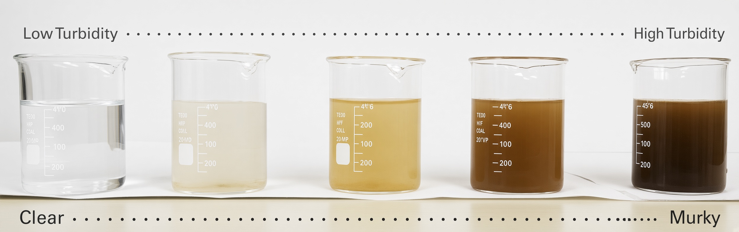
Excessive suspended solids can negatively affect fish health and system performance. Fine particles may irritate or clog the gills, increase physiological stress, reduce growth rates, and create favourable conditions for opportunistic pathogens. Suspended particles can also reduce water clarity, interfere with fish behaviour and feeding, decrease the effectiveness of UV disinfection by shielding microorganisms from ultraviolet light, and increase the biological oxygen demand as organic matter decomposes.
In recirculating aquaculture systems (RAS), solids management is a critical design and operational consideration. The goal is to remove particles as quickly as possible after they are produced, before they break down into dissolved wastes that are more difficult to remove. Effective solids control typically relies on self-cleaning tank hydraulics, central drains, swirl separators, radial flow settlers, drum filters, microscreens, and regular sludge removal. Well-designed hydraulics help transport particles rapidly to treatment units while preventing accumulation in tanks and pipework.
Particle size is also important. Larger particles are generally easier to remove mechanically, whereas fine particles may remain suspended for long periods and require advanced filtration, foam fractionation, or polishing treatment. As particles break apart through pumping and recirculation, removal becomes increasingly difficult, making rapid solids capture a key objective in modern RAS design. See drum filters, sludge handling and the mass balance under dissolved oxygen (TSS per kg feed).
Values below refer to TSS in mg/L. Acceptable levels vary with species, life stage, system design and production intensity. Turbidity (e.g. NTU) often correlates with TSS but is not the same measurement - only compare values in the same unit. Orientation, not a permit value.
| TSS (mg/L) | General interpretation |
|---|---|
| < 5 | Excellent |
| 5–15 | Good |
| 15–30 | Acceptable |
| 30–50 | Elevated — monitor closely |
| > 50 | Poor solids control |
| > 100 | Likely to impact fish health and system performance |
Teaching orientation for intensive culture. Salmonids and hatcheries often aim toward the lower end. Always check against your standard and UV requirements (UVT).
Not all species are equally sensitive to solids. Salmonids (rainbow trout, salmon, Arctic char) are often "primadonnas": they want clear, oxygen-rich water and react early to gill irritation and stress. Carp are more robust in ponds. Catfish and mudfish (e.g. Clarias) cope better with murkier, organic-rich water. Shrimp sit in between — intensive tank/RAS prefer clearer water, while pond culture often runs murkier. Figures are teaching approximations for an upper preferred TSS (mg/L), not culture protocols.
| Species group | Approx. upper preferred TSS | Clarity preference | Comment |
|---|---|---|---|
| Salmonids (trout, salmon, char…) | ~10–15 mg/L | Very clear | Primadonnas — gills and stress-sensitive |
| Shrimp — intensive tank / RAS | ~20–30 mg/L | Clear | UV, visibility and gills benefit from low TSS |
| Shrimp — pond / semi-intensive | ~40–60 mg/L | Moderate–murky | Algae and clay common; manage oxygen and sediment |
| Carp | ~50–80 mg/L | Tolerates murk | Classic pond species; robust but not "dirty = good" |
| Catfish / mudfish (e.g. Clarias) | ~100–150 mg/L | Murky OK | Best murky/organic tolerance in this comparison |
Same linear thinking as the bar chart. Intensive RAS usually aims lower than ponds for the same species. Fry and hatchery tighter than grow-out.
Approx. upper preferred (mg/L TSS)
Bars show an approximate upper preferred TSS (mg/L) for “good culture water”, same linear scale 0–150. Salmonids want clear water; carp tolerate more; catfish/mudfish and many pond shrimp cope with murkier water. Intensive RAS usually aims lower than ponds. Not a species protocol or permit value.
© 2026 DABCE AB
Teaching point: design solids control for the species — a rainbow trout RAS needs fast, fine filtration; a Clarias pond can live with more murk if oxygen and gills stay under control. "Tolerates murky" does not mean ignore filters and UV when the system needs clear water.
In short: remove particles early, whole and dry - before they become dissolved problems for gills, UV, oxygen and the biofilter. See drum filters, disc filters, sludge and UV.
DABCE can help with a review, checklists and short training.
Contact DABCE — contact@dabce.seSources/overview (selection): Timmons & Ebeling, Recirculating Aquaculture Systems; Summerfelt, solids removal in freshwater RAS; FAO aquaculture engineering resources; Lekang, Aquaculture Engineering. Orientation - not species-specific limits or permits.
Oxidation-Reduction Potential (ORP), sometimes called redox potential, is a measurement of the water's ability to oxidise or reduce substances. It is expressed in millivolts (mV) and is widely used in aquaculture as an indirect indicator of water cleanliness, organic loading, and the effectiveness of oxidising treatments such as ozone.
In RAS, ORP is most commonly associated with ozone systems. When ozone is added to water, it oxidises dissolved organic matter, improves water clarity, reduces colour, enhances microsolids removal, and can help lower microbial loads. As ozone dosage increases, ORP generally rises. For this reason, ORP is often used as a control parameter for automated ozone dosing systems.
While elevated ORP can indicate improved water quality, excessively high ORP values may be harmful to fish. Exposure to residual ozone or excessive oxidation can damage gill tissue, irritate skin and eyes, increase stress, and in severe cases cause mortality. For this reason, ozone treatment is normally applied in dedicated contact chambers or side-stream treatment loops, followed by degassing and residual ozone destruction before the water returns to the fish culture tanks.
ORP should not be viewed as a direct measurement of ozone concentration. Many factors influence ORP, including dissolved oxygen, pH, temperature, organic loading, salinity, and other oxidising or reducing compounds present in the water. ORP is therefore best used as a trend indicator and process control tool rather than as an absolute water quality parameter.
Modern intensive RAS facilities commonly use ORP monitoring to optimise ozone dosing while maintaining safe conditions for fish. Proper system design, residual ozone destruction, and continuous monitoring are essential when operating ozone treatment systems. See ozone systems, UV and turbidity/TSS.
Values below are approximate mV bands often mentioned in RAS practice. Target values vary with species, system design, salinity and ozone strategy. Always interpret ORP together with residual ozone measurements (where used) and overall water quality — not alone. Orientation, not a permit value.
| ORP (mV) | General interpretation |
|---|---|
| < 200 | High organic loading, low oxidation capacity |
| 200–250 | Typical untreated aquaculture water |
| 250–325 | Good water quality in many RAS systems |
| 325–375 | Often observed during controlled ozone treatment |
| 375–425 | Elevated — requires careful monitoring |
| > 425 | Potential risk of residual ozone exposure |
| > 450 | Generally considered unsafe for direct fish exposure |
Reference electrode and calibration affect the reading. Only compare measurements on the same farm and with the same probe/type. Trend over time is more useful than a single number.
In short: ORP is a useful steering wheel for ozone and a rough "cleanliness" trend — but it is not an ozone sensor and not harmless when it spikes. Design so fish never meet residual ozone.
DABCE can help with a review, checklists and short training.
Contact DABCE — contact@dabce.seSources/overview (selection): Summerfelt, ozonation and UV in RAS; Timmons & Ebeling, Recirculating Aquaculture Systems; Lekang, Aquaculture Engineering; Colt, water quality for aquaculture. Orientation — not species-specific limits or dosing protocols.
Drum filters (microscreens) are the most common primary solids step in modern RAS and semi-flow facilities. A rotating drum with mesh (often about 40–90 µm) removes faeces, feed waste and other suspended particles as water passes outward or inward through the cloth.
When the mesh blinds, backwash starts — usually high-pressure spray nozzles and/or level or pressure control. Backwash water becomes a concentrated sludge stream that continues to settling, thickening or other sludge handling.
Finer mesh clears water more but raises backwash volume, headloss and wash frequency. Coarser mesh lets more fines through to biofilters and UV. Choose micron rating from species, feed, downstream steps and available sludge handling — not “as fine as possible”.
Orientation — not a supplier selection. Capacity depends on mesh, load, temperature and water quality.
See also
Disc filters use stacked discs (often grooved or micro-structured) as filter media. Water passes between or through the discs while particles are retained. When the filter blinds, the disc pack is backwashed or opened so solids can be flushed away.
Disc filters are a compact alternative to drum filters for some flows and footprints — especially where floor space is limited or several smaller units fit better than one large drum.
See also
Sand filters are classic deep-bed filtration: water passes through a bed of sand (or similar media) where particles lodge in the pores. The technology is well known in municipal and industrial water treatment; in aquaculture it is often used for polishing, effluent treatment or continuous sand filters (e.g. DynaSand class) rather than as the sole solids step in heavily loaded RAS.
Size on filtration rate (m/h), raw-water quality and target outlet TSS/turbidity. Monitor headloss, backwash frequency and media level. In FlowFarm-like semi-flow concepts, continuous sand filtration is often used as an integrated biostage/particle step — see flow-through.
See also
Bead filters use floating plastic beads as both mechanical filter media and biofilm surface. Water is pushed or pumped through the bed; particles are trapped between beads while nitrifying bacteria can grow on the surfaces.
The technology is common in smaller RAS, hatcheries and hobby/research systems where one compact unit should combine solids capture and some biological treatment. In large commercial RAS, separate drum filters plus dedicated biofilters (MBBR, fixed bed, trickling) are more often the standard.
See also
A Moving Bed Biofilm Reactor (MBBR) is one of the most common biological filtration technologies used in modern aquaculture. The process consists of thousands of small plastic carrier elements suspended in a continuously mixed and aerated tank. These carriers provide a large protected surface area where beneficial bacteria form a biofilm.
The primary role of an MBBR is nitrification: ammonia (NH₃/NH₄⁺) → nitrite (NO₂⁻) → nitrate (NO₃⁻). By continuously removing toxic ammonia and nitrite, the biofilter helps maintain a stable environment for fish and enables much higher stocking densities than would otherwise be possible. See Ammonia / TAN and nitrite.
See also
Water containing dissolved waste enters the reactor and flows around freely moving plastic carriers. The biofilm growing on the carriers contains nitrifying bacteria that convert ammonia into nitrite and nitrite into nitrate.
Aeration, mechanical mixing or the water flow itself (pumped circulation through the reactor) keeps the carriers in motion, ensuring:
Unlike fixed-media biofilters, MBBRs do not rely on stationary packing material and are generally less prone to channeling and fouling.
MBBRs have become a standard component in many RAS and intensive flow-through systems because they combine simplicity with high treatment capacity. Advantages include:
For these reasons, MBBRs are commonly used in facilities producing salmon, trout, char, tilapia, shrimp and many other cultured species.
MBBRs do not remove waste for free. Nitrification consumes oxygen and alkalinity. For every amount of ammonia converted, significant quantities of oxygen are required and alkalinity is gradually consumed. As a result, biofilter performance depends on adequate dissolved oxygen, stable pH, sufficient alkalinity, appropriate temperature and healthy bacterial populations. Poor oxygenation or low alkalinity can quickly reduce nitrification efficiency. See dissolved oxygen, alkalinity and pH.
The calculator below goes from peak feed to TAN load, biofilm area needed, media volume, reactor size, oxygen and mixing air. Pick a scenario (salmon/trout, sturgeon, tilapia, clarias) to set TAN yield and conversion per m² available area — you can change the value. Set mixing air to 0 if pumped circulation moves the carriers. Not a design calculation — media, temperature, salinity and load govern real conversion.
Typical culture temperature about 10–16 °C. Conservative conversion per m².
© 2026 DABCE AB
A newly installed MBBR contains little or no nitrifying biomass. The biofilm must develop over time as bacteria colonise the carriers. During start-up, ammonia removal is initially limited, nitrite spikes are common, feeding may need to be restricted and water quality requires close monitoring. Biofilter maturation can take weeks to months depending on temperature, water chemistry, bacterial seeding and loading rates. See nitrite.
In Recirculating Aquaculture Systems (RAS), the MBBR is often regarded as the biological heart of the facility. A typical RAS process train may include:
Fish tanks
↓
Solids removal
↓
Degassing
↓
MBBR
↓
Oxygenation
↓
Back to fish tanks
The order can vary (biofilter and degassing sometimes swap places). The biofilter works continuously and directly determines how much feed the system can process and therefore how much fish biomass the farm can support. Operators often monitor TAN, nitrite, nitrate, pH, alkalinity and dissolved oxygen as indicators of biofilter performance. See RAS.
| Technology | Typical strength |
|---|---|
| MBBR | Robust, simple, scalable |
| Fixed-bed biofilter | High efficiency, compact footprint |
| Trickling filter | Excellent CO₂ stripping and oxygen transfer |
| Bead filter | Solids removal and biofiltration combined |
| Fluidised sand filter | Very high surface area and treatment capacity |
Each technology has advantages, and many modern RAS facilities combine several treatment processes. Orientation, not a ranking.
Although MBBRs are highly effective, they are not a complete water-treatment solution. They do not directly remove solids, carbon dioxide, phosphorus, colour or most dissolved organic compounds. These parameters require additional processes such as drum filters, settling systems, protein skimmers, degassing towers and ozone or UV treatment.
The MBBR is the engine room of biological filtration. As long as oxygen, alkalinity and carrier surface area are sufficient, an MBBR can provide highly reliable nitrification and support large fish biomasses. Most biofilter problems are caused not by the carriers themselves, but by insufficient oxygen, inadequate alkalinity, poor solids management, or attempting to feed the system faster than the bacteria can grow.
Sources/overview (selection): Timmons & Ebeling, Recirculating Aquaculture; established RAS practice on moving-bed biofilters. Orientation, not a design calculation. See also RAS, Ammonia / TAN, nitrite, alkalinity and dissolved oxygen.
Fixed bed biofilters are biological filters that use stationary media to provide a large protected surface area for nitrifying bacteria. The media may consist of plastic modules, structured packing, gravel, rock, lava media, synthetic materials or other high-surface-area substrates that remain fixed in place while water flows through them.
Like all biological filters, their primary purpose is nitrification: ammonia (NH₃/NH₄⁺) → nitrite (NO₂⁻) → nitrate (NO₃⁻). By converting toxic ammonia and nitrite into less toxic nitrate, fixed bed biofilters help maintain water quality and support higher fish stocking densities. See Ammonia / TAN and nitrite.
See also
Water passes through stationary filter media where biofilms containing nitrifying bacteria grow on the media surfaces. As water flows through the biofilter, ammonia is converted to nitrite and nitrite to nitrate. Oxygen and alkalinity are consumed. Because the media remains fixed, biofilms can develop large and stable bacterial populations with excellent treatment capacity. Many fixed bed systems operate under low-energy conditions and require little or no mechanical mixing — flow through the bed is often enough.
Fixed bed biofilters have been used in aquaculture for decades and remain popular in hatcheries, small RAS, flow-through farms, recirculation systems and public aquaria. Advantages include:
Because the biofilm is protected within the media structure, these filters can support large bacterial populations in a relatively compact footprint.
The biggest challenge with fixed bed biofilters is fouling. If suspended solids are not removed before the biofilter, waste particles become trapped within the media and gradually block water flow. Potential consequences include reduced hydraulic performance, channeling and dead zones, oxygen depletion within the media, reduced nitrification rates, increased maintenance and formation of anaerobic zones.
For this reason, fixed bed biofilters are normally installed after effective solids removal such as drum filters, settling systems, microscreens or hydrocyclones. Good solids management is often the difference between a highly efficient fixed bed biofilter and a poorly performing one.
Like all nitrifying systems, fixed bed biofilters require dissolved oxygen, alkalinity, stable pH and suitable temperature. Nitrification continuously consumes both oxygen and buffering capacity. If oxygen or alkalinity becomes limiting, ammonia removal declines, nitrite may accumulate and efficiency falls. See dissolved oxygen, alkalinity and pH.
The same model as for MBBR: peak feed → TAN load → area needed → media volume → bed size. Fixed-bed defaults are a lower specific area (structured plastic, orientation) and a higher fill, with air 0 because the bed is not normally mixed. Conversion per m² is the same variable as in the MBBR calculator — fouling reduces the real area. Not a design calculation.
Typical culture temperature about 10–16 °C. Conservative conversion per m².
© 2026 DABCE AB
| Feature | Fixed bed | MBBR |
|---|---|---|
| Media movement | Stationary | Moving |
| Surface area | Very high | High |
| Energy demand | Low | Moderate |
| Solids sensitivity | Higher | Lower |
| Risk of clogging | Higher | Lower |
| Expansion | Less flexible | Easily expanded |
| Maintenance | More cleaning | Generally lower |
Both perform the same biology. Fixed beds often achieve excellent nitrification; MBBRs are typically more forgiving when feed loads fluctuate or solids removal is imperfect.
Fixed bed biofilters are particularly common in hatcheries where feed loads are moderate, water quality is closely controlled, stable operation is prioritised and tank biomass is relatively predictable. Many trout, salmon and char hatcheries have successfully used fixed bed biofilters for decades.
The goal is always the same: maximising surface area while maintaining effective water flow and oxygen supply. Specific area differs greatly between gravel and structured plastic — enter the right figure in the calculator.
Fixed bed biofilters do not directly remove solids, carbon dioxide, phosphorus, colour or dissolved organic compounds. Additional treatment is typically required, including drum filtration, degassing, oxygenation, UV and sometimes ozone. Poor solids removal can eventually force shutdown and cleaning of the biofilter.
A fixed bed biofilter can provide extremely efficient nitrification, but only if solids are removed before the water reaches the media. Good solids removal protects the biofilter. Poor solids removal eventually turns the biofilter into a solids filter. The greatest strength is the large protected bacterial surface. The greatest weakness is fouling.
Sources/overview (selection): Timmons & Ebeling, Recirculating Aquaculture; established hatchery and RAS practice. Orientation, not a design calculation. See also MBBR, Ammonia / TAN, nitrite, alkalinity and dissolved oxygen.
A trickling filter is a biological filter where water is distributed over a stationary bed of media while air circulates freely through the filter. As water trickles downward across the media surface, a biofilm of nitrifying bacteria removes dissolved nitrogen compounds from the water.
Like other biofilters, the primary purpose is nitrification: ammonia (NH₃/NH₄⁺) → nitrite (NO₂⁻) → nitrate (NO₃⁻). Trickling filters are unique because they provide both biological filtration and highly effective gas exchange in the same unit. See Ammonia / TAN, carbon dioxide and dissolved oxygen.
See also
Water is sprayed, distributed or dripped across media with a large surface area. As water flows over the biofilm, ammonia is converted into nitrite, nitrite into nitrate, oxygen is absorbed from the air and carbon dioxide (CO₂) is stripped from the water. Unlike submerged biofilters, the media is exposed to both air and water, allowing the bacteria direct access to atmospheric oxygen.
Common media include structured plastic packing, random plastic media, lava rock, synthetic biofilter modules and other high-surface-area materials. The packing must stay open enough for air to pass.
Trickling filters are widely used because they combine several treatment processes into one unit. Advantages include:
In many aquaculture systems, the CO₂ removal can be almost as valuable as the nitrification itself.
One of the greatest strengths of a trickling filter is gas exchange. As water is broken into thin films and droplets, carbon dioxide diffuses into the air, additional oxygen enters the water and excess nitrogen gas may also be reduced. This makes trickling filters particularly attractive in RAS where fish continuously produce large amounts of carbon dioxide.
High CO₂ can reduce growth, worsen feed conversion, increase stress and reduce oxygen-uptake efficiency. A properly designed trickling filter helps address both ammonia and CO₂ at the same time. See carbon dioxide, dissolved oxygen and pH.
Like fixed-bed biofilters, trickling filters perform best when solids have already been removed. Excess solids can coat surfaces, restrict airflow, promote unwanted bacterial growth, reduce nitrification and increase maintenance. They are therefore usually located after drum filters, settling systems, microscreens or other primary solids removal.
Nitrification still consumes dissolved oxygen and alkalinity. Oxygen transfer is often excellent, but alkalinity consumption remains significant. Monitor TAN, nitrite, pH, alkalinity and dissolved oxygen. See alkalinity and Ammonia / TAN.
The same model as for MBBR and fixed bed: peak feed → TAN → area → media volume → tower volume. Defaults are a lower specific area (open packing so air can pass) and air 0 (natural draft). The calculator sizes nitrification volume — not CO₂ stripping, hydraulic loading or tower height. Not a design calculation.
Typical culture temperature about 10–16 °C. Conservative conversion per m².
© 2026 DABCE AB
In recirculating systems they are used as stand-alone biofilters, combined nitrification and degassing units, polishing stages after MBBRs or supplemental CO₂ removal. Typical trains:
Fish tanks → drum filter → trickling filter → oxygenation → fish tanks
Fish tanks → drum filter → MBBR → trickling filter → oxygenation → fish tanks
The exact configuration depends on production goals and system design. See RAS and MBBR.
| Feature | Trickling filter | MBBR |
|---|---|---|
| Nitrification | Excellent | Excellent |
| CO₂ removal | Excellent | Limited |
| Oxygen transfer | Excellent | Good |
| Moving parts | Few | Needs mixing/aeration |
| Solids sensitivity | Moderate | Lower |
| Footprint | Often larger (height) | More compact |
| Energy use | Low | Moderate |
Many modern RAS farms combine both: MBBRs for high nitrification capacity and trickling filters for additional gas exchange.
Although highly effective, trickling filters do not directly remove suspended solids, phosphorus, colour or most dissolved organic compounds. They also require sufficient height and airflow, which may increase building requirements. In cold climates, heat losses can be greater than in submerged systems because of the large air–water interface.
An MBBR is primarily a nitrification reactor. A trickling filter is both a nitrification reactor and a degassing system. If ammonia and carbon dioxide are both challenges, a properly designed trickling filter can address both at the same time. For many farms it is not just a biofilter, but part of the facility's gas-management strategy.
Sources/overview (selection): Timmons & Ebeling, Recirculating Aquaculture; established RAS practice on trickling filters and gas exchange. Orientation, not a design calculation. See also MBBR, fixed bed, carbon dioxide and dissolved oxygen.
Protein skimmers, also known as foam fractionators, remove dissolved and fine particulate organic matter by generating large numbers of small air bubbles. Organic compounds attach to the bubble surfaces and are carried upward as foam, which is collected and removed from the system.
Protein skimming is widely used in marine aquaculture, public aquariums and marine RAS because seawater naturally supports efficient foam formation. In freshwater systems the process is generally much less effective, although some specialised freshwater applications exist.
See also
Many dissolved organic compounds contain both hydrophilic and hydrophobic regions and therefore accumulate at the air–water interface. When fine air bubbles are injected, dissolved organics attach to bubble surfaces, the bubbles rise, foam forms at the surface and the foam is removed as concentrated waste. The process is often called foam fractionation because organics become concentrated within the foam phase.
By removing these materials before they break down, skimmers can reduce the load on downstream treatment.
Organic waste constantly enters aquaculture systems through feed, fish excretions, mucus and microbial activity. If these organics accumulate they can increase oxygen demand (BOD), promote bacterial growth, reduce water clarity, increase biofouling and contribute to off-flavours. Protein skimmers remove a portion of these compounds before they decompose.
The effectiveness of foam fractionation increases significantly with salinity. Seawater ions strengthen bubble stability and improve foam formation. As a result, marine RAS, hatcheries, public aquariums and shrimp or marine fish systems often use skimmers as standard equipment. In freshwater salmonid systems they are generally much less efficient and therefore less commonly used. See salinity.
Protein skimmers are frequently combined with ozone. Ozone can break down dissolved organics, improve water clarity, increase skimmer efficiency, reduce colour and turbidity and lower microbial loads. In marine RAS, ozone contact is often followed by a protein skimmer that removes oxidised organic material. See ozone and UV.
Typically after solids removal and before biological filtration. Simplified trains:
Fish tanks → drum filter → protein skimmer → biofilter → oxygenation → fish tanks
Fish tanks → drum filter → ozone contact → protein skimmer → biofilter
The exact arrangement depends on system design. See drum filters and MBBR.
Protein skimmers do not replace biological filtration. They do not directly remove ammonia (TAN), nitrite, nitrate, carbon dioxide or most dissolved salts. Those need biofilters, degassing, water exchange or denitrification. View skimmers as organic-load reduction, not a complete water-treatment solution.
Removal is in practice governed by bubble area × contact time × the amount of organic matter. The larger the total bubble area and the longer the contact, the more organic can be removed. Do not size on system volume alone.
Skimmer size ∝ feed mass × organic load — not ∝ water volume. Two farms with the same volume but different feed rates can need very different skimmers.
Start from the mass load, not the tank volume. A simplified chain: feed → organic waste → solids removal → remaining foamable material → skimmer → foam concentrate.
L_skim = F × f_org × f_diss × f_avail. F is peak feed (kg/d), f_org the share leaving the fish as organic, f_diss the dissolved or very fine share after mechanical filtration, f_avail the share that is surface-active and practically foamable. The last factor is the most uncertain — not all DOC is foamable. Use the highest realistic daily feed, not the annual average, and also check the peak hour.
Hydraulic check: Qs = V × N / 24 is treatment flow from system volume and turnovers per day — a check, not the primary sizing. Contact time tc = V_effective / Qs. Air/water RA/W = Q_air / Qs. Bubble area grows roughly with air flow / bubble diameter. The calculator below takes the feed load and shows load, flow, contact time, air ratio and an indicative contact volume. Not a supplier selection.
Seawater: better foam. f_avail start 0.30 (0.38 with ozone).
Loop volume = tanks + recycle this skimmer serves, not the skimmer body. Flow 0 = calculate loop volume × turnovers / 24.
© 2026 DABCE AB
Biofilters remove dissolved nitrogen. Protein skimmers remove dissolved organics. Size first on how much organic is produced (feed load), not on how many cubic metres of water the system holds. The chain is: feed → DOC → bubble area → foam → removal. Final selection against representative water quality, salinity, feed load and supplier or pilot data.
Sources/overview (selection): Timmons & Ebeling; established marine RAS and aquarium practice on foam fractionation. f_org / f_diss / f_avail and specific load are start values, not verified removal rates. Orientation, not a design calculation. See also ozone, UV, salinity and MBBR.
Ozone (O₃) is one of the strongest oxidants used in aquaculture and water treatment. It is widely applied in Recirculating Aquaculture Systems (RAS), hatcheries and marine production systems to improve water quality, reduce dissolved organic matter, improve water clarity and support microbial control. Ozone is also widely used to sterilise supply and effluent water in aquaculture systems.
Unlike chlorine, ozone leaves no long-term disinfectant residual because it naturally decomposes back into oxygen. This makes it attractive for aquaculture, but it also means ozone must be generated on-site and used immediately. Ozone is highly unstable and therefore generated locally rather than stored.
When properly engineered and operated, ozone can significantly improve water quality and production stability. When poorly applied, it can damage fish, destroy biofilter performance, create toxic residual oxidants and present serious safety risks to personnel. Higher ozone concentrations can cause tissue damage, stock mortalities and risks to biofilters.
As production intensity increases, organic wastes accumulate within the system. While drum filters and biofilters remove solids and nitrogen compounds, they do not efficiently remove all dissolved organics and fine colloidal particles. Ozone is often used as an additional process step to manage these compounds. Ozone is used to remove organic carbon, turbidity, algae, colour, odour and taste, and to improve system stability.
Potential benefits include:
Many operators notice ozone first as “clearer water”, but the underlying benefits often extend throughout the entire treatment train.
Ozone is a highly reactive molecule consisting of three oxygen atoms. The third oxygen atom is weakly bound and readily reacts with other compounds. This makes ozone a powerful oxidising agent. The instability of ozone is what gives it its treatment effectiveness.
When ozone enters water it reacts with:
Many of these reactions occur very rapidly. In addition to direct oxidation, ozone may initiate secondary oxidation reactions that further improve water quality.
Ozone should generally not be applied directly into culture tanks. Instead, it is normally used in a dedicated treatment loop. Water is usually treated in a side-stream and returned only after ozone has reacted or been removed. Side-loop treatment and dedicated contact systems are commonly used to avoid direct fish exposure.
Typical components include:
One of the most important practical benefits of ozone is its interaction with foam fractionation systems. Ozone can alter dissolved organic compounds, improve particle aggregation, increase skimmer efficiency, improve water clarity and reduce yellowing compounds. Many marine RAS facilities combine protein skimmers and ozone treatment specifically because the two technologies complement each other.
Ozone and UV are often treated as competing technologies, but they are frequently complementary. Ozone can improve UV performance by reducing dissolved organics that absorb ultraviolet light. Improved UV transmittance is a recognized outcome of ozonation.
A common approach is: mechanical filtration → ozone treatment → foam fractionation → UV treatment → culture system. This sequence can improve overall treatment efficiency and biosecurity.
Water colour and turbidity are common challenges in intensive production systems. Over time dissolved organics accumulate and create yellow-brown water colour, lower UV penetration, reduced visibility and increased organic loading. Ozone breaks down many of these compounds and improves visual water quality. The result is often better visibility, improved UV effectiveness and reduced organic load.
Ozone can support biofilter performance indirectly by reducing organic loading. However, excessive ozone exposure can damage nitrifying bacteria. Potential problems include loss of nitrification capacity, reduced ammonia and nitrite conversion and biofilter instability.
For this reason, ozone is usually applied upstream of residual removal and not directly to biofilters. The goal is improved water quality without exposing biofilter bacteria to harmful residual oxidants.
Freshwater applications are generally more straightforward. Ozone primarily reacts with organic matter and microorganisms. Risks still exist, but chemistry is usually easier to manage than in marine systems. Even in freshwater systems: residual ozone must not reach fish, ORP should be monitored, ozone demand varies with water quality, and dosing should be adjusted gradually.
Marine ozone treatment requires significantly greater caution. Seawater contains naturally high levels of bromide. Ozone reacts rapidly with bromide and forms secondary oxidants, often referred to as ozone-produced oxidants. These compounds may persist longer than ozone itself and can create biological risks if not properly controlled. Fish can sometimes be affected even when no measurable ozone remains.
These secondary oxidants may include:
Because of this chemistry, seawater ozonation is more complex, marine species may be exposed to secondary oxidants, conservative operation is essential and residual destruction is critical. Safe seawater ozone treatment depends on controlled contact time, off-gas handling, oxidant management and careful monitoring.
ORP (Oxidation Reduction Potential) is commonly used for process control. When oxidation increases, ORP generally rises. However, ORP is not a direct ozone measurement. ORP responds to many chemical conditions within the water and should be interpreted as an indicator rather than an ozone concentration measurement.
ORP is best viewed as a process control parameter, an early warning indicator and a trend measurement — not a direct ozone sensor or a replacement for good system design. See ORP.
Ozone is highly effective but must be treated as an industrial oxidant. Ozone gas can be hazardous to personnel and should never be allowed to accumulate in enclosed spaces. High atmospheric ozone concentrations are hazardous to health.
Ozone often provides the greatest benefit in intensive RAS, hatcheries, smolt facilities, marine RAS, high-density production, systems with low water exchange and facilities requiring high water clarity. The technology becomes increasingly attractive as water reuse rates increase.
Ozone is not simply a disinfection tool. It is a water quality management technology. In most successful aquaculture applications, ozone improves system performance by reducing dissolved organics, improving water clarity, supporting foam fractionation and lowering microbial pressure. The goal is not maximum oxidation. The goal is controlled oxidation.
Fish should never be exposed to free ozone, marine systems require special attention due to bromide chemistry, and residual destruction should always be part of the treatment train. When properly designed and conservatively operated, ozone can be one of the most powerful tools available for maintaining stable water quality in intensive aquaculture systems.
Orientation — not a dosing protocol or species-specific limits. Verify design against supplier guidance, ORP practice and local water chemistry (especially bromide in seawater).
See also
Ultraviolet (UV) disinfection is one of the most widely used water treatment technologies in aquaculture. Unlike chemical disinfectants, UV inactivates microorganisms using light rather than oxidation or chemical residuals.
Modern aquaculture facilities use UV systems to reduce pathogen pressure, protect hatcheries, improve biosecurity and support stable production. UV is commonly applied to intake water, make-up water, recirculation loops and effluent streams depending on the farm’s biosecurity objectives.
One of the biggest advantages of UV is that it leaves no chemical residual in the water. There is no chlorine, ozone or disinfectant remaining after treatment. This makes UV particularly attractive ahead of biofilters, fish tanks and sensitive life stages such as eggs, larvae and fry.

Most aquaculture UV systems operate using UV-C light at approximately 254 nm. When microorganisms pass through the reactor, UV radiation damages DNA and RNA, preventing replication. The organism may still physically exist, but it can no longer reproduce and infect new hosts.
UV can affect bacteria, viruses, fungal spores, algae, protozoa and some parasite stages. The effectiveness depends on both the organism and the dose delivered. A UV reactor does not sterilise water in the strict sense. Instead, it provides a specific level of inactivation depending on UV dose and reactor performance.
One of the most common mistakes is focusing on lamp wattage rather than UV dose. The important parameter is UV dose (mJ/cm²). Dose is determined by UV intensity, exposure time, reactor hydraulics, water quality and lamp condition.
A large UV unit can still deliver poor treatment if flow is too high or water quality is poor. Conversely, a properly sized UV unit can achieve excellent performance with relatively modest power consumption. When evaluating a UV system, always ask what UV dose is being delivered at the actual operating flow — not how many watts the lamp consumes.
Many UV suppliers describe performance using UV intensity or UV dose at a specific location within the reactor, typically expressed as mJ/cm² — the flux of UV photons at a certain distance or point. From a disinfection perspective this is entirely reasonable because microorganisms passing through the reactor receive a specific UV exposure based on intensity and residence time.
For barrier-treatment applications such as intake water, hatcheries and effluent disinfection, delivered dose remains the primary design parameter. In these applications the objective is often to achieve a defined level of pathogen inactivation during a single pass through the UV reactor. Both mJ/cm² and related design values matter.
However, recirculating aquaculture systems (RAS) are fundamentally different. In a RAS, the same water continuously circulates through treatment equipment. Water may pass through a UV system dozens or even hundreds of times before a microorganism has sufficient time to reproduce significantly. From a biological perspective, the question is often not only “What UV dose does one pass receive?” but also: how much UV energy is deposited into the recirculating water volume over time?
For this reason, many process engineers find it useful to think in terms of UV energy input per cubic metre of system water, UV power relative to recirculating flow, total UV treatment intensity relative to system volume, or UV energy relative to feed load or biomass. These metrics do not replace traditional UV dose calculations, but they can simplify comparisons between different reactor designs and focus on the biological dose–effect in the system.
The biological reality is that in many RAS facilities, water returns to the UV system much faster than bacteria, viruses or many other microorganisms can reproduce. As a result, total system exposure over repeated passes may become just as important as single-pass dose.
A simple distinction is often useful:
The most useful engineering approach is often to understand both perspectives. A reactor may have excellent single-pass validation data, yet provide limited overall impact if only a small fraction of system water reaches it. Conversely, a modest reactor treating a very large fraction of recirculating flow may provide substantial biological benefits at the system level.
Water quality has a major influence on UV performance. Before UV light can inactivate microorganisms, it must reach them. UVT describes how much UV light passes through the water. Low UVT may be caused by dissolved organic matter, water colour, fine particles, turbidity, algal cells, iron or manganese. Poor UVT can dramatically reduce delivered dose. Two systems with identical UV equipment may achieve completely different results if one has poor water clarity.
UV works best on clean water. Particles can shield microorganisms from UV radiation. This means bacteria or parasites embedded within particles may survive treatment even when UV dose appears adequate. For this reason, UV systems are typically installed downstream of drum filters, disc filters, microscreens, clarifiers, foam fractionators and ozone systems. The cleaner the water entering the UV reactor, the more effective the UV system becomes.

Many hatcheries treat all incoming water with UV before it enters production. Benefits include reduced pathogen introduction, improved biosecurity and more predictable production conditions. This is one of the most common UV applications worldwide.
Eggs, larvae and fry are highly susceptible to disease. UV treatment is therefore widely used in egg incubation systems, fry systems, broodstock facilities and live feed production. Many hatcheries consider UV one of their primary disease-prevention barriers.
In RAS facilities UV may be used to reduce microbial load, improve water hygiene, protect sensitive production stages and support overall biosecurity. Because UV leaves no residual, water can immediately return to the fish after treatment.
Some facilities apply UV treatment before water discharge — for pathogen control, biosecurity, environmental protection and regulatory compliance.
UV and ozone are frequently used together. Rather than competing technologies, they often complement each other. Ozone can reduce colour, improve UVT and remove dissolved organics. UV can then provide microbial control, inactivate pathogens and act as a final barrier before culture water returns to fish. Many high-performance RAS facilities employ both technologies as part of a multi-barrier approach.
UV can also operate as part of Advanced Oxidation Processes (AOP). Examples include UV + ozone, UV + hydrogen peroxide, and UV + ozone + peroxide. These systems create highly reactive hydroxyl radicals. Potential applications include dissolved organic removal, advanced water polishing, reduction of refractory compounds and improved water reuse. AOP systems are considerably more complex than standard UV disinfection and usually require specialist design and operation.
Most UV systems contain a quartz sleeve that separates the lamp from the water. Light must pass through this sleeve to reach the water. Fouling may occur from biofilms, scale, calcium deposits, iron deposits and organic matter. Even small amounts of fouling can significantly reduce UV performance. Modern units often use automatic wipers, chemical cleaning and UV intensity monitoring. Regular inspection remains essential.
UV lamps degrade over time. A lamp that still lights up may no longer produce sufficient UV output. This is why commercial UV systems are usually maintained based on operating hours, UV intensity measurements and manufacturer recommendations — not simply on whether the lamp still appears functional. Many facilities lose significant UV performance because aging lamps are not replaced on schedule.
Modern UV systems increasingly include UV intensity sensors, UVT monitoring, flow monitoring, alarm systems, data logging and SCADA integration. Monitoring allows operators to verify that the required dose is actually being delivered. Without monitoring, operators often assume performance rather than measure it.
For many farms, UV represents one of the simplest and most reliable biosecurity technologies available.
Some viruses, protozoa and parasite stages may require significantly higher doses than routine bacterial control. For this reason, UV should be viewed as one barrier within a broader biosecurity strategy rather than a complete disease-prevention solution.
The effectiveness of a UV system depends far more on delivered dose than installed wattage. Clean water, good UV transmittance, proper hydraulic design, functioning lamps and regular maintenance are what determine performance.
UV suppliers often sell reactors based on delivered dose. Aquaculture operators ultimately care about biological results. For intake-water disinfection, validated UV dose is usually the key design parameter. For recirculating systems, it is often equally important to consider how much UV energy is continuously being applied to the total water volume and microbial population within the system. The reactor treats water once. The system treats the water hundreds of times. Understanding the difference helps explain why two facilities with similar UV reactors may experience very different biological outcomes.
In practice, the most successful aquaculture facilities treat UV as a process system rather than a lamp. Filter first, measure UVT, size for the required dose with a safety margin, monitor performance continuously and maintain lamps, quartz sleeves and sensors on schedule. When properly designed and operated, UV remains one of the most effective and widely used biosecurity barriers in modern aquaculture.
Orientation — not a validated log-reduction protocol or supplier selection. Verify dose, UVT and flow against current reactor data and target organisms.
See also
Oxygen cones (e.g. Speece cone / oxygen cone) are pressurized contactors where water and pure oxygen meet under elevated pressure. That raises oxygen solubility and gives high transfer efficiency — common when pure O₂ is used in RAS, raceways and intensive land-based systems.
Monitor DO before/after, oxygen pressure and leaks. Calibrate DO sensors at critical points. The cone does not replace good hydraulics or a sound overall oxygen strategy (air first, pure O₂ as additive where it pays).
See also
An LHO (Low Head Oxygenator) oxygenates water at low hydraulic head. Water is distributed over chambers or packing where oxygen (or oxygen-enriched gas) contacts the water without needing the high pump pressures of a deep oxygen cone. That makes LHOs energy-efficient in many RAS designs.
Many facilities first maximise air-side uptake in degassers/trickling, then use an LHO or cone for the final O₂ boost. See degassers, oxygen cones and oxygen demand.
See also
Degassers (CO₂ strippers) remove carbon dioxide and can simultaneously increase air-side oxygen uptake. Common designs are cascades, packed columns and other air/water contactors where water is broken into films and droplets while air flows counter- or co-currently.
In RAS, fish continuously produce CO₂. High levels reduce growth and welfare long before DO becomes critical. Degassing is therefore often as important as pure oxygen dosing.
See also
Aeration supplies air (~21% O₂) to water via diffusers, surface aerators, blowers, venturis or cascades. It is the most common and usually cheapest way to raise DO — but gas transfer per flow is lower than with pure oxygen, so intensive systems need more turnover or complementary O₂.
Blowers and surface aerators can dominate the power bill. Maintain diffusers (fouling cuts transfer), avoid unnecessary over-aeration, and control against DO sensors with sensible deadbands. Always compare lifecycle cost with pure oxygen — see CAPEX/OPEX and oxygen supply.
See also
Heat pumps move heat from a source (effluent, raw water, hall air, ground or waste heat) into culture water or the building. In cold climates, heating can be one of the largest OPEX items in land-based farming — so heat recovery is often critical for energy economics.
Heat pumps raise CAPEX but can cut OPEX sharply over the facility lifetime — a classic CAPEX/OPEX trade-off. See temperature, CAPEX & OPEX and sustainability.
See also
Chillers remove heat from culture water or hall air when temperature would otherwise rise above the species comfort zone. Demand is high in warm climates, in tightly insulated RAS halls with high internal heat load, and for cold-preferring species such as Arctic char.
Cooling is energy-intensive. Minimise internal heat (pump efficiency, insulation, ventilation) before sizing chillers. See heat pumps, temperature and energy under CAPEX/OPEX.
See also
Monitoring is the basis for safe farming around the clock - whether the site is an earthen pond, raceway, net pen or full RAS. Without knowing what is happening in the water, you only react when the fish already show stress. With the right measurements, problems can be caught early: falling oxygen, a sudden temperature swing, a stopped pump, a full settler or a failed intake.
Whatever the production system, two parameters are practically indispensable: dissolved oxygen (DO) and temperature. Oxygen drives respiration, growth and survival - and changes quickly with feed, density, algal blooms, ice, pump failure or heat. Temperature drives metabolism, oxygen demand, immunity and the species comfort zone (e.g. Arctic char vs tilapia). Without some form of measurement of these, you are flying blind.
How you measure differs a lot. On a simple pond farm, a handheld DO/temperature probe a few times a day, plus eyes and experience, may be enough. On a commercial RAS you expect continuous sensors, PLC/SCADA, trends, SMS/email alarms and often redundant measuring points. In between - raceways, semi-flow-through, net pens - sites often combine spot checks with fixed sensors at critical points.
Large volume, natural primary production and strong day-night swings (algal photosynthesis raises DO by day; night risk of low DO). Measurement often focuses on DO and temperature at surface and depth, Secchi depth, and sometimes pH/alkalinity. Continuous sensors become more common at higher density, but many farms still rely on handheld checks, night watches and aeration started manually or via simple DO switches.
Water quality is driven strongly by intake flow and source condition. It is important to track temperature and DO on inlet and outlet water, plus flow (too little flow means oxygen risk and ammonia risk). Handheld checks can suffice on small sites; larger raceways and hatcheries often have fixed DO/temp sensors, flow switches and alarms on pump or intake failure. Solids and turbidity from the source may need turbidity or simple optical checks.
Fish live in the surrounding water body - measurement is about understanding the environment around the pen, not a closed loop. Typically: temperature profiles, DO (especially in summer stratification, algal blooms or ice), sometimes current, salinity and weather. On modern marine sites, buoys, underwater sensors and feed/camera monitoring are common; simpler lake cages may still use daily handheld checks and observation. Alarms for low oxygen or storms are more "environmental warning" than "pump trip".
Here monitoring is a process-safety issue. The system is tightly coupled: pump failure, biofilter trouble, rising CO2 or low oxygen can escalate in minutes. Standard is continuous sensors for DO, temperature, pH, often ORP/redox, level, flow and pressure; plus 24/7 alarms to staff. SCADA/PLC controls oxygen, valves and emergency modes. Spot checks (TAN, nitrite, nitrate, alkalinity, CO2) complement - some online, many still lab or handheld kits. The higher the reuse, the more critical the measurement becomes.
Typical measuring points on more advanced farms: DO and temperature in tanks and critical return lines; pH in the biofilter loop; flow and level in sumps; alarms on power, emergency power and oxygen reserve. Calibration, sensor placement (dead zones vs representative mixing) and spare sensors matter as much as "having a sensor".
Better monitoring is not only fewer emergency trips - it enables higher density with maintained welfare, lower feed waste, faster troubleshooting and documentation for permits and customers. Data from DO, temp, flow and feed can link to growth models, energy control and early disease warning. Remote monitoring cuts the need for constant presence on distant pens or inland sites, while responsibility still requires someone who can act when the alarm sounds.
The potential is greatest where risk is fast and value high: RAS, hatcheries, high density and species with a narrow temperature window. But pond and cage farms also gain by moving from handheld-only checks to at least continuous DO/temp with alarms. The next steps - digital twins, AI feed control and automatic oxygen/flow optimisation - always rest on the same base: reliable measurements, especially oxygen and temperature.
Sensors for DO, pH, temperature, level, flow and alarms - with SCADA/PLC and SMS/email where needed - are the basis for safe operation. Match measuring level to system, density and staffing; do not under-invest in oxygen and temperature.
DABCE TyrFlow™ is a triple-redundant sensing system with edge computing - developed among other uses for aquaculture, where reliable measurement and fast local processing are critical. Three independent measuring paths and computation near the sensors give more robust data, fewer false alarms and continued function even when cloud connectivity is limited. Contact DABCE for more on TyrFlow in farming, RAS and other demanding water applications.
Aquaculture facilities are highly vulnerable to power outages — whether hatchery, RAS, raceway, pond with aeration, net pen with feed/cameras or shrimp farm. Even short interruptions can lead to oxygen depletion, loss of circulation, reduced filtration performance, temperature instability, and significant stock losses. Reliable backup systems are therefore considered essential infrastructure in all intensive aquaculture — not merely an operational convenience.
A typical backup strategy uses multiple layers of protection. Design is based on the acceptable time-to-failure of critical life-support functions: aeration/oxygen, circulation pumps, biofilters, monitoring and communication are usually prioritised. Required backup duration may range from a few minutes in grid-stable areas to several days in remote locations.
Uninterruptible Power Supplies (UPS) provide immediate short-term power for PLCs, sensors, SCADA systems, communication equipment, alarms, and critical controls while larger backup systems start. Without a UPS the control system dies the instant the grid fails — even if the generator starts within a minute.
Diesel or natural gas generators are the most common solution for extended outages. Generators are typically sized to operate life-support systems such as pumps, blowers, oxygen generators, feeding equipment, and control systems. Automatic Transfer Switches (ATS) detect outages and automatically transfer loads from the utility grid to backup generators or batteries.
Battery Energy Storage Systems (BESS) are becoming increasingly common. Lithium-ion battery banks can bridge generator startup, support critical loads for several hours, and integrate with renewable energy systems. Some facilities use batteries as the primary backup with generators as secondary support. Solar PV combined with batteries is increasingly used for remote and off-grid facilities — usually still supplemented by generators for long-duration reliability.
Emergency oxygen reserves are often considered more important than backup power itself. Liquid oxygen (LOX) tanks, compressed oxygen cylinders, or oxygen cones supplied from reserve storage can maintain fish or shrimp survival during prolonged power failures even if full water circulation cannot be maintained. Size oxygen against peak feed/biomass and worst-case DO demand — see dissolved oxygen and oxygen demand.
For intensive aquaculture, backup power and emergency oxygen are risk management: they protect animal welfare, production assets and business continuity. See RAS, hatchery, monitoring systems, SCADA and oxygen.
DABCE can help with a review, checklists and short training.
Contact DABCE — contact@dabce.seSources/overview (selection): established practice in intensive aquaculture (RAS, hatchery, land-based, pens with critical loads); Timmons & Ebeling and others on process safety. Sizing of generators, BESS and LOX is site- and load-specific — orientation, not electrical engineering design.
Egg incubators are used to provide stable and controlled conditions during the sensitive early life stages of fish. Their purpose is to maximize hatching success, reduce disease risk, and ensure uniform development from fertilized eggs to first-feeding larvae or fry.
Successful incubation depends on maintaining the correct water temperature, dissolved oxygen level, flow rate, and water quality for the species being cultured. Most incubators are kept in low light or darkness, as fish eggs naturally develop in shaded environments and excessive light can increase stress and reduce hatch quality in some species.
Water flow serves several functions. It delivers oxygen, removes carbon dioxide and metabolic waste products, prevents stagnant zones, and helps keep eggs clean. Flow must be strong enough to maintain good water quality but gentle enough to avoid damaging delicate eggs.
Dead or unfertilized eggs should be removed regularly. These eggs are often quickly colonized by fungi such as Saprolegnia, which can spread to healthy eggs and cause significant losses. Modern hatcheries may use manual inspection, siphoning, automated sorting systems, or image-based monitoring to identify and remove non-viable eggs. See also egg disinfection and biosecurity.
Different incubator designs are used depending on the species:
Temperature has a major influence on development speed. Warmer water generally accelerates embryonic development, while colder water slows it down. However, temperatures outside the species-specific optimum range may increase deformities, mortality, or poor larval quality. For this reason, many hatcheries use temperature-controlled water systems to maintain precise conditions throughout incubation. See temperature and dissolved oxygen.
Modern commercial hatcheries increasingly monitor egg survival, hatch rate, temperature, dissolved oxygen, pH, flow rate, and developmental progress using digital sensors and automated alarm systems. Early detection of problems can significantly improve productivity and biosecurity. Hatcheries are also extremely sensitive to power loss - see backup power systems.
Good egg incubation practices often determine the performance of the entire production cycle. High-quality eggs, stable environmental conditions, careful handling, and effective disease prevention are among the most important factors for achieving strong fry and fingerlings.
Incubator sizing is usually based on annual fry production, egg-to-fry survival, and how long eggs stay in the incubator. A simple chain:
The table gives approximate orders of magnitude for egg size, packing density, degree-days to hatch and typical incubation temperature. Strain, broodstock status, salinity and hatchery practice cause large differences — use as orientation, not a protocol.
| Species | Egg Ø (mm) | Eggs/L (approx.) | °D to hatch | Temp (°C) |
|---|---|---|---|---|
| Atlantic salmon | 5.5–7.0 | 6 000–8 000 | 400–550 | 6–10 |
| Rainbow trout | 4.5–6.0 | 7 000–10 000 | 280–420 | 8–12 |
| Arctic char | 4.5–5.5 | 8 000–12 000 | 450–650 | 4–8 |
| Brown trout | 4.0–6.0 | 7 000–10 000 | 350–500 | 6–10 |
| Coho salmon | 5.0–6.5 | 6 000–9 000 | 450–550 | 6–10 |
| Chinook salmon | 6.0–8.0 | 5 000–7 000 | 500–700 | 5–10 |
| Sturgeon | 2.5–4.0 | 20 000–50 000 | 70–150 | 15–22 |
| Common carp | 1.2–1.8 | 100 000–200 000 | 60–90 | 20–28 |
| Grass carp | 1.5–2.0 | 80 000–150 000 | 40–80 | 22–30 |
| Tilapia | 2.0–3.0 | 30 000–80 000 | 70–120 | 26–30 |
| Pike-perch (zander) | 1.3–1.8 | 100 000–180 000 | 80–120 | 12–18 |
| European perch | 1.0–1.5 | 150 000–300 000 | 80–120 | 10–18 |
| Sea bass | 1.0–1.3 | 300 000–700 000 | 70–110 | 13–18 |
| Sea bream | 0.9–1.1 | 500 000–1 000 000 | 40–80 | 16–22 |
| Atlantic cod | 1.2–1.5 | 250 000–500 000 | 90–150 | 4–8 |
| Halibut | 3.0–4.0 | 20 000–60 000 | 250–500 | 5–8 |
| Whiteleg shrimp (L. vannamei) | — | millions of larvae / L-scale* | — | 28–31 |
| Giant river prawn (M. rosenbergii) | — | millions of larvae / L-scale* | — | 28–31 |
* Shrimp are often incubated/larval-reared at much higher density and in different units than salmonid eggs — do not compare directly with salmonid eggs/L. Teaching ranges; strain and hatchery practice govern.
Orders of magnitude for hatchery batches. A “batch” can mean a hatch window or a production round — not a global standard.
| Species | Typical hatchery batch (orientation) |
|---|---|
| Arctic char | ~0.1–5 million eggs |
| Rainbow trout | ~0.5–20 million eggs |
| Atlantic salmon | ~1–50+ million eggs |
| Sturgeon | ~10,000–5 million eggs |
| Tilapia | ~10,000–500,000 eggs |
| Carp | ~100,000–50 million eggs |
| Sea bass | ~1–50+ million eggs |
| Sea bream | ~1–100+ million eggs |
| Shrimp | ~10–500 million larvae |
Scale varies enormously with company, market and species. Use as order-of-magnitude in early sizing.
The calculator below uses mid-range values from the table for common presets (salmon, trout, Arctic char, tilapia, carp). Adjust eggs/L, °D and temperature to your protocol.
Incubator type
© 2026 DABCE AB
Example (worked illustration, Arctic char preset): 1,000,000 fry/year, 80% survival → 1,250,000 eggs/year. At 6 °C and 550 °D → about 92 days; simultaneous inventory ≈ 314,000 eggs; at 10,000 eggs/L ≈ 31 L; with 1.5× spare ≈ 47 L active incubation volume across trays or units. Try the same numbers in the calculator. Oxygen-based flow sizing (Q = M_O₂ / ΔDO) can become limiting near hatch — see dissolved oxygen.
The calculator above effectively assumes steady year-round production: eggs are incubated more or less continuously so inventory and tank capacity can be sized on “eggs at once”. In reality salmonids in general are driven by seasonal breeding cycles — rainbow trout, Atlantic salmon, Arctic char, brown trout and others — as long as the broodstock environment is not controlled with light and temperature. Wild stocks and farmed broodfish under natural light/temp spawn in a limited window. Without deliberate planning the hatchery gets a large egg pulse over a few weeks and then long periods with empty trays. That loads incubators, staff, fry tanks and later grow-out unevenly — and means the “tonnes per year” in a spreadsheet do not match the actual biology.
If you want to level the flow of fry and food fish over the year, there are essentially two strategic paths (often combined):
Milt (sperm) from salmonids can be cryopreserved (frozen) with established technique and thawed when needed. Unfertilised eggs are far more sensitive: egg banking by deep-freezing ova is not standard to the same extent as for milt, although research and specialised methods continue. In practice, “freezing the biology” therefore often means: store frozen milt, and/or hold fertilised eggs in controlled, slow development (cold water, planned °D budget) so hatch is spread — more “tempered delay” than a freezer. Some hatcheries also buy eyed eggs from several suppliers or seasons to fill gaps. The same logic applies to rainbow trout, salmon and Arctic char: without light-/temperature-controlled broodstock (or bought eggs from several windows), egg supply clumps — planning egg supply and incubation temperature is then critical if you want to avoid a single annual peak.
The second path is to control when broodstock spawn. Salmonids — rainbow trout, Atlantic salmon, Arctic char and others — respond strongly to light (photoperiod) and temperature. Under natural light and seasonal temperature, spawning is therefore seasonal. With controlled light regimes — and often temperature — one can shift, compress or spread spawning: e.g. several brood groups out of phase, out-of-season eggs, or more than one spawn season per year in closed systems. That is a standard tool in many commercial salmonid hatcheries, not only for one species. In land-based farming (RAS/semi-flow) the reason is especially clear: you want to fill tanks evenly year-round to use CAPEX, labour and market capacity.
In practice many commercial salmonid hatcheries combine both: controlled broodstock to get eggs when needed, frozen milt as backup, and incubation at a chosen temperature to fine-tune hatch date within the °D window. The sizing calculation (steady inventory) then becomes a target to approach — not a law of nature. Without egg banking or cycle control you must instead size incubators, fry tanks and staff for the peak season and accept lower utilisation the rest of the year.
Example: a salmonid farm (rainbow trout, salmon or Arctic char) that wants food fish every month needs either light-/temperature-controlled broodstock with groups out of phase, bought/eyed eggs from several windows, and/or planned incubation time — otherwise hatch and grow-out clump. See temperature, life cycle, biosecurity and species pages. Orientation — not a breeding protocol.
DABCE can help with a review, checklists and short training.
Contact DABCE — contact@dabce.seSources/overview (selection): FAO aquaculture development guidelines; Wedemeyer, Fish Hatchery Management; Piper et al., Fish Hatchery Management; Timmons & Ebeling, Recirculating Aquaculture Systems; established practice on photoperiod/broodstock and milt cryopreservation in salmonids. The sizing calculator is orientation — not a hatchery project or species-specific protocols/doses.
Heath trays, also known as vertical incubators, are among the most widely used egg incubation systems in salmonid hatcheries. Multiple trays are stacked vertically, allowing large numbers of eggs to be incubated within a relatively small floor area. Water typically enters at the top of the stack and flows downward through each tray, providing oxygen and carrying away waste products.
The design offers excellent space efficiency and is particularly suited for species with relatively large demersal eggs, such as Atlantic salmon, rainbow trout, Arctic char, brown trout, and Pacific salmon species. Individual trays can be removed for inspection, grading, disinfection, or egg picking without disturbing the entire incubation system.
Typical loading densities range from several thousand to tens of thousands of eggs per tray, depending on egg size and hatchery practices. A single Heath stack may hold hundreds of thousands of eggs, making the system highly scalable for both small hatcheries and commercial facilities producing millions of fry annually.
Advantages include high egg density, simple construction, easy inspection, good water distribution, and proven performance over decades of commercial use. However, careful management of flow distribution and routine removal of dead eggs are important to prevent fungal outbreaks and maintain high survival rates. See also egg incubators, egg disinfection and biosecurity.
| Parameter | Orientation |
|---|---|
| Water flow | ~2–10 L/min per tray |
| Egg loading | ~5,000–50,000 eggs per tray |
| Dissolved oxygen (DO) | > 8 mg/L (typically near saturation) |
| Temperature | Species dependent; salmonids commonly about 4–12 °C |
| Common hatchery scale | ~0.1–10+ million eggs |
| Stack geometry (typical data) | Often 8 trays/stack; height about 1.6–2.0 m |
Teaching ranges. Flow, load and temperature depend on species, egg size and hatchery standard — not fixed rules.
Number of trays ≈ (number of eggs / eggs per tray) × safety factor, where the safety factor is often about 1.1–1.5 (spare, uneven loading, picking). Number of stacks ≈ trays / trays per stack (e.g. 8).
Example: 1,000,000 Arctic char eggs, 25,000 eggs/tray, safety factor 1.25 → trays = 1,000,000 / 25,000 × 1.25 = 50 trays. With 8 trays/stack ≈ 7 stacks (rounded up). The same logic is used in the calculator under Egg incubators (choose stacked trays).
DABCE can help with a review, checklists and short training.
Contact DABCE — contact@dabce.seSources/overview (selection): Wedemeyer, Fish Hatchery Management; Piper et al., Fish Hatchery Management; established salmonid hatchery practice; see also Egg incubators. Orientation — not a supplier specification or protocol.
Fry and larval tanks are used after hatching and yolk sac absorption, when young fish begin exogenous feeding and become fully dependent on environmental conditions and nutrition. This stage is often one of the most sensitive in aquaculture, as small changes in water quality, feeding, light, or stocking density can strongly affect survival, growth, and later production performance.
Larval tanks are typically shallow and designed with gentle hydraulics to minimize stress and ensure that weak-swimming larvae can easily access feed. Water flow must provide sufficient oxygen and waste removal without creating excessive currents that force larvae to expend energy or become trapped against screens.
The transition to first feeding is a critical developmental milestone. Larvae must locate and consume feed before yolk reserves are exhausted. In many marine species, live feeds such as rotifers and Artemia are used during the earliest stages before gradual introduction of formulated feeds. Freshwater species such as salmonids typically transition directly to commercial starter diets after yolk sac absorption.
Light intensity and photoperiod are important design and operational considerations. Many species require specific light regimes to locate feed, regulate behaviour, and support growth. Excessive light can increase stress, while insufficient illumination may reduce feeding efficiency. Hatcheries often use programmable lighting systems. Stocking density must be carefully controlled. High densities can improve space utilization but may increase competition, stress, oxygen consumption, disease transmission, and size variation. Frequent grading is often required to reduce cannibalism in species such as perch, pike-perch, barramundi, and many marine fish.
Modern fry-rearing systems increasingly incorporate automated feeding, oxygen control, image-based monitoring, and environmental sensors for more consistent results. See monitoring systems, dissolved oxygen and feed.
| Parameter | Orientation |
|---|---|
| Water depth | 0.2–1.5 m |
| Tank volume | 50–10 000 L |
| Dissolved oxygen | > 80–90% saturation |
| Exchange rate | ~0.5–10 tank volumes/day (species dependent) |
| Light | Species and life-stage dependent |
| Marine larvae | ~20–200 larvae/L |
| Salmonid fry | ~5–50 kg/m³ |
| Tilapia fry | ~1,000–10,000 fry/m³ |
Teaching ranges. Fry and larvae are sensitive — aim toward the safer side of the ranges. Not a protocol.
Volume ≈ number of fry / target density (fish/m³), or volume ≈ biomass / target biomass density (kg/m³). Example: 100,000 salmon fry at 10,000 fry/m³ → 10 m³. Alternatively 200 kg fry at 20 kg/m³ → 10 m³.
Fish use the water column and swim. Shrimp are largely bottom-dwelling: they walk, graze, hide and moult. Design therefore differs clearly even though both are reared in “tanks”.
Fish tanks are usually sized as density in kg/m³ (or fish/m³). For shrimp — especially larger juveniles and grow-out — the limit is often animals/m² or kg/m² because animals occupy the bottom. A shrimp tank may therefore be shallower and wider than a fish tank holding similar biomass. Many systems add extra surface: meshes, sheets, net curtains, artificial seaweed or biofloc structures — several times the floor area. For fish, extra surface is rarely relevant except as biofilter media.
Fish tanks may use circular flow for swimming stimulus and self-cleaning. Shrimp tanks need gentler hydraulics: avoid strong currents, protect moulting animals, avoid feed in corners. Flow is mainly for oxygen and solids. Faeces and feed sink quickly; bottom deposits favour Vibrio. Hence: central drains, sloped floors, bottom flushing, frequent sludge removal. During moulting shrimp are vulnerable to cannibalism, mechanical damage and water-quality swings — habitat, stable salinity, alkalinity and calcium/magnesium become critical (often monitored as carefully as DO).
Intensive shrimp culture can reach animal densities impossible for most fish. Orientation: extensive ponds a few shrimp/m²; semi-intensive often tens to ~150/m²; intensive lined ponds and indoor RAS much higher (hundreds–thousands/m² depending on stage). Fish are more often limited earlier by oxygen and swimming behaviour. Shrimp feed mainly on the bottom, more slowly and continuously — multiple daily feeds, feed trays, automatics, acoustic sensors and cameras are common. Biofloc (BFT) is widespread in shrimp: microbial aggregates consume ammonia and are grazed by shrimp; FCR and water exchange can improve. Fish RAS often aims to remove suspended solids, whereas biofloc intentionally maintains them.
Simple shrimp nursery sizing: area (m²) ≈ number of shrimp / target density (shrimp/m²). Example: 100,000 nursery shrimp at 500/m² → 200 m². Fish systems are normally sized primarily from tank volume and biomass density instead.
In short: fish tanks are generally designed around water volume and swimming behaviour; shrimp tanks often around bottom area, surface area, feeding behaviour and moulting biology. That is why modern indoor shrimp farms frequently use shallow raceways, lined ponds, stacked nursery tanks and large amounts of artificial substrate, while salmon, trout, char, sea bass and tilapia are more commonly reared in circular tanks, raceways or cages designed around volume and hydraulic performance.
DABCE can help with a review, checklists and short training.
Contact DABCE — contact@dabce.seSources/overview (selection): Timmons & Ebeling, Recirculating Aquaculture Systems; FAO hatchery/nursery and shrimp culture guidelines; Wedemeyer, Fish Hatchery Management; Summerfelt & Vinci; Boyd & McNevin; Treece & Yates; Avnimelech, Biofloc Technology. Orientation — not species-specific protocols or density limits.
Egg disinfection is a standard biosecurity measure in many hatcheries and is commonly performed when fertilized or eyed eggs arrive from external suppliers. The goal is to reduce the risk of introducing bacterial, fungal, viral, or parasitic pathogens into the hatchery. Treatment is typically performed shortly after egg arrival, during transfer between facilities, or before eggs enter the hatchery water system.
Industry standard for routine baths of eyed salmonid eggs: iodophor (iodine-based disinfectant). Alternatives such as H₂O₂ and ozone are used in some cases — see below. No doses on this page.
Iodophor-based disinfectants are the most widely used treatment for routine disinfection of eyed salmonid eggs and remain the industry standard in many hatcheries worldwide. They are effective against many surface-associated pathogens while being relatively safe for fish eggs when applied according to the manufacturer's instructions. Disinfection does not sterilize the egg interior but helps reduce contamination on the egg surface and shell.
Correct concentration, exposure time, water quality, and thorough rinsing are essential. Excessive dosage or prolonged exposure can damage developing embryos and reduce hatch rates. Follow species-specific recommendations, veterinary requirements and local rules — this page does not give doses.
Hydrogen peroxide is used in some hatcheries and applications, among other things to control fungal growth (Saprolegnia) on eggs. It breaks down into water and oxygen and leaves no long-term residue. It is not the global standard for routine salmonid egg baths in the same way as iodophor, but can be a complement or alternative where protocols and rules allow.
Ozone is an extremely powerful oxidant and disinfectant. It is common for hatchery and RAS water treatment (make-up, bio-barrier, clarity) — see ORP and ozone systems — but it is rarely the first choice for a direct egg bath. Residual ozone has a narrow safety margin and can quickly damage egg membranes and embryos.
Good egg disinfection should be combined with supplier health certification, quarantine, equipment sanitation, water treatment, and regular hatchery health monitoring. Disinfection reduces risk but cannot compensate for poor hygiene or infected broodstock. Particular attention when eggs move between regions or countries — an important pathway for disease transmission.
Key principle: the best programme combines healthy broodstock, clean water, biosecurity procedures and careful egg handling. No disinfectant can compensate for poor hatchery hygiene. Especially common in hatcheries for Atlantic salmon, rainbow trout, Arctic char, brown trout, sturgeon and many marine finfish traded internationally. See Heath trays, egg incubators, biosecurity, ORP and ozone.
Pick method and egg stage. The tool sets orientation C and t, computes CT = C × t and builds a simple checklist. Always adjust against an approved product, label and veterinary advice — defaults are teaching start values for salmonids, not legal requirements.
Aquarium keepers: the same principles can of course apply to home breeding, but it is usually more important to simply separate eggs/fry into a small, clean holding or hatching container (with gentle flow or aeration) — away from adult fish, predators and dirt in the main tank. A disinfection bath is rarely the first step in an aquarium; biosecurity and a clean, stable environment for the young are.
Orientation for salmonids in hatcheries — not a product label or veterinary protocol. Adjust C and t against an approved product. Never exceed manufacturer limits.
Suggested SOP (checklist)
© 2026 DABCE AB
DABCE can help with a review, checklists and short training.
Contact DABCE — contact@dabce.seSources/overview (selection): FAO aquaculture biosecurity guidelines; WOAH (OIE) Aquatic Animal Health Code; Wedemeyer, Fish Hatchery Management; Piper et al., Fish Hatchery Management; Timmons & Ebeling; research/practice on H₂O₂ and ozone in hatcheries. SOP defaults are orientation — follow approved products, label and veterinary advice.
Atlantic salmon (Salmo salar) is an anadromous species that hatches and grows in freshwater before migrating to the ocean, where it spends most of its grow-out phase. Atlantic salmon is the dominant aquaculture species in Norway, Scotland, the Faroe Islands, Iceland, Canada and Chile, accounting for the majority of global farmed salmon production. Traditionally produced in sea cages, the industry is increasingly adopting land-based systems for smolt production, post-smolt rearing and, in some cases, full grow-out to harvest size.
Atlantic salmon performs best in cool, well-oxygenated water. Growth rates are strongly influenced by temperature, with optimal growth typically occurring between approximately 10 and 16 °C. Elevated temperatures increase metabolism, oxygen demand and disease risks, while prolonged exposure to warm water can lead to reduced feed intake, stress and mortality. Temperature control is therefore a critical design consideration in both freshwater and seawater RAS.
Modern RAS salmon production requires strict management of water quality. Key parameters include dissolved oxygen (DO), carbon dioxide (CO₂), ammonia (TAN), nitrite, alkalinity, pH, salinity and suspended solids. Atlantic salmon are particularly sensitive to elevated CO₂ concentrations, making degassing systems an essential component of recirculating facilities. Efficient oxygenation and robust biofiltration are required to support high biomass densities while maintaining fish welfare and growth performance.
Biosecurity is a major driver behind land-based salmon farming. Closed systems can reduce exposure to sea lice, pathogens, harmful algal blooms and environmental fluctuations that affect open-net pen production. However, this requires rigorous disinfection protocols, quarantine procedures, water treatment systems and continuous monitoring to prevent disease outbreaks within the facility.
Atlantic salmon remains the benchmark species for large-scale recirculating aquaculture technology and has been a major driver of innovation in biofiltration, oxygenation, water treatment, automation, fish health monitoring and backup life-support systems. Today, salmon RAS facilities range from small freshwater hatcheries producing a few million smolts annually to industrial-scale land-based farms targeting tens of thousands of tonnes of harvest-size fish per year.
Atlantic salmon has one of the longest production cycles in aquaculture. Exact duration depends on strain, temperature, feeding, photoperiod and whether production is in traditional sea cages or RAS. The tables below are typical ranges under favourable conditions — not guaranteed protocols.
| Stage | Size / weight | Typical duration |
|---|---|---|
| Egg incubation | Fertilised egg → hatch | ~2–3 months (depends on °D and temp) |
| Alevin (yolk sac) | Newly hatched | Weeks to swim-up |
| First-feeding fry | ~0.2–1 g | Weeks–months |
| Fingerling / parr | ~5–80 g | Months in freshwater |
| Smolt | ~80–200 g (classic) | ~8–18 months from egg |
| Large smolt / post-smolt | ~0.3–1 kg | ~16–22 months from egg |
| Seawater grow-out or grow-out RAS | to 3–7 kg | +12–24 months after smolt |
| Harvest fish | ~3–5 kg typical | ~24–36 months from egg |
| Large premium harvest | ~5–7 kg | ~30–36+ months from egg |
Ranges under favourable conditions. Strain, temperature, density and health change the timeline.
Approximate progression under favourable conditions (orientation):
| Time from fertilisation | Approximate size |
|---|---|
| Day 0 | Fertilised egg |
| 2–3 months | Hatch |
| 4–5 months | First-feeding fry |
| 7–9 months | 5–10 g parr |
| 10–14 months | 30–80 g parr |
| 12–18 months | 80–200 g smolt |
| 16–22 months | 0.5–1.0 kg post-smolt |
| 24–30 months | 3–5 kg harvest fish |
| 30–36 months | 5–7 kg premium harvest |
Modern post-smolt RAS often delivers 300–1,000 g before sea transfer; classic hatcheries often deliver 80–150 g smolt. Fully land-based food fish omits the marine phase.
This long production cycle is one reason salmon farmers place strong emphasis on biosecurity, backup power, oxygen supply and water quality management, as losses at any stage can represent years of biological investment.
The tool estimates time from start phase/weight to target weight (based on the orientation growth curve above) and proposes a simplified tank/stage chain toward an annual production target. Density, survival and number of tank sizes are adjustable. Orientation — not bankable facility design.
1. Time from start to target weight
Approximate growth (orientation)
Curve uses the same orientation data as the time calculator; tempo scales the x-axis. Logarithmic weight axis. Orientation — not a feed-control growth model.
2. Production chain toward annual target
H/W = water depth ÷ diameter (round) or flat–flat span (octagon). Optimal default 0.30 ≈ Ø:depth 3.3:1 (typical circular RAS tanks). Lower = flatter/larger footprint; higher = deeper/narrower.
Density (kg/m³) by fish size — adjust to strategy. More stages ⇒ shorter time per tank and sizing to exit weight ⇒ lower total volume.
Stages in the chain
| Stage | Weight (g) | Months | Fish in stage (avg) | Biomass (t) | kg/m³ | Volume (m³) |
|---|
Suggested tank plan
| Tank class | Stage | Days in tank | Unit volume | Depth | Area / tank | Diameter / span | Units | Class volume |
|---|
3. Layout generator (to scale, area = CAPEX) (Experimental)
Packing biased to the golden ratio (φ≈1.618): D+1.0 m cells, grid/shelf and a segment meta-grid so the hall is not one long thin strip.
Packing runs as JS in the browser (grid + shelf). Shared service D+1.0 m. Dashed circle = 0.5 m service zone. Orientation — not construction documentation.
© 2026 DABCE AB
DABCE can help with a review, checklists and short training.
Contact DABCE — contact@dabce.seSee also
Sources/overview (selection): established industrial practice for Salmo salar (cages, smolt, post-smolt, land-based RAS); Timmons & Ebeling and others on RAS; public industry statistics (Norway etc.). Growth and density figures are orientation — strain, temperature, feed and health govern real time and volume.
Rainbow trout (Oncorhynchus mykiss) is one of the world’s most widely farmed salmonids. It is robust, has a mature feed and market chain, and is grown in raceways, ponds, cages, semi-flow-through and RAS. Unlike Atlantic salmon, trout is usually farmed for the whole cycle in fresh or brackish water — portion (pan-size) or larger food fish depending on market.
Optimal growth typically sits around 10–16 °C. Trout tolerates somewhat higher temperatures than Arctic char but still responds to heat with higher oxygen demand and stress. In RAS, stable temperature, high DO, controlled CO₂ and good solids handling are the keys to high density with maintained welfare.
Compared with Atlantic salmon the cycle to portion size is shorter, and seawater smoltification is not standard in Nordic inland farming. Large fish (2–4+ kg) appear in premium and fillet markets. See also FlowFarm for semi-flow concepts.
Exact duration depends on strain, temperature (~12–16 °C often favourable), feed and density. Tables are typical ranges under favourable conditions — not protocols.
| Stage | Size / weight | Typical duration |
|---|---|---|
| Egg incubation | Fertilised egg → hatch | ~3–5 weeks (depends on °D/temp) |
| Alevin / yolk sac | Newly hatched | Weeks to swim-up |
| First-feeding fry | ~0.2–1 g | Weeks |
| Fingerling | ~5–50 g | Months |
| Juvenile | ~50–200 g | Months |
| Portion / pan-size | ~250–450 g | ~10–16 months from egg |
| Large food fish | ~1.5–3 kg | ~16–24 months from egg |
| Very large / premium | ~3–4+ kg | ~22–30+ months from egg |
Ranges under favourable conditions. Strain, temperature and health govern real time.
| Time from fertilisation | Approximate size |
|---|---|
| Day 0 | Fertilised egg |
| ~1 month | Hatch |
| ~2 months | First feeding |
| ~4 months | 5–10 g fingerling |
| ~6 months | 30–50 g |
| ~9 months | 100–200 g |
| ~12 months | ~300–400 g portion |
| ~16 months | ~1–1.5 kg |
| ~20 months | ~2–3 kg |
| ~26 months | ~3–4 kg |
Rule of thumb: portion fish often about 10–16 months from egg; large fish another 6–12+ months. Orientation.
Same type of tool as for Atlantic salmon, but with trout’s faster growth curve and end products (portion / large fish). Density, survival, tank classes and layout generator included. Orientation — not bankable design.
1. Time from start to target weight
Approximate growth (orientation)
Curve uses the same orientation data as the time calculator; tempo scales the x-axis. Logarithmic weight axis. Orientation — not a feed-control growth model.
2. Production chain toward annual target
H/W = water depth ÷ diameter (round) or flat–flat span (octagon). Optimal default 0.30 ≈ Ø:depth 3.3:1 (typical circular RAS tanks). Lower = flatter/larger footprint; higher = deeper/narrower.
Density (kg/m³) by fish size — adjust to strategy. More stages ⇒ shorter time per tank and sizing to exit weight ⇒ lower total volume.
Stages in the chain
| Stage | Weight (g) | Months | Fish in stage (avg) | Biomass (t) | kg/m³ | Volume (m³) |
|---|
Suggested tank plan
| Tank class | Stage | Days in tank | Unit volume | Depth | Area / tank | Diameter / span | Units | Class volume |
|---|
3. Layout generator (to scale, area = CAPEX) (Experimental)
Packing biased to the golden ratio (φ≈1.618): D+1.0 m cells, grid/shelf and a segment meta-grid so the hall is not one long thin strip.
Packing runs as JS in the browser (grid + shelf). Shared service D+1.0 m. Dashed circle = 0.5 m service zone. Orientation — not construction documentation.
© 2026 DABCE AB
DABCE can help with a review, checklists and short training.
Contact DABCE — contact@dabce.seSee also
Sources/overview (selection): established practice for Oncorhynchus mykiss (raceway, pond, cage, RAS); Timmons & Ebeling; Piper et al. Growth figures are orientation — strain, temperature, feed and health govern real time and volume.
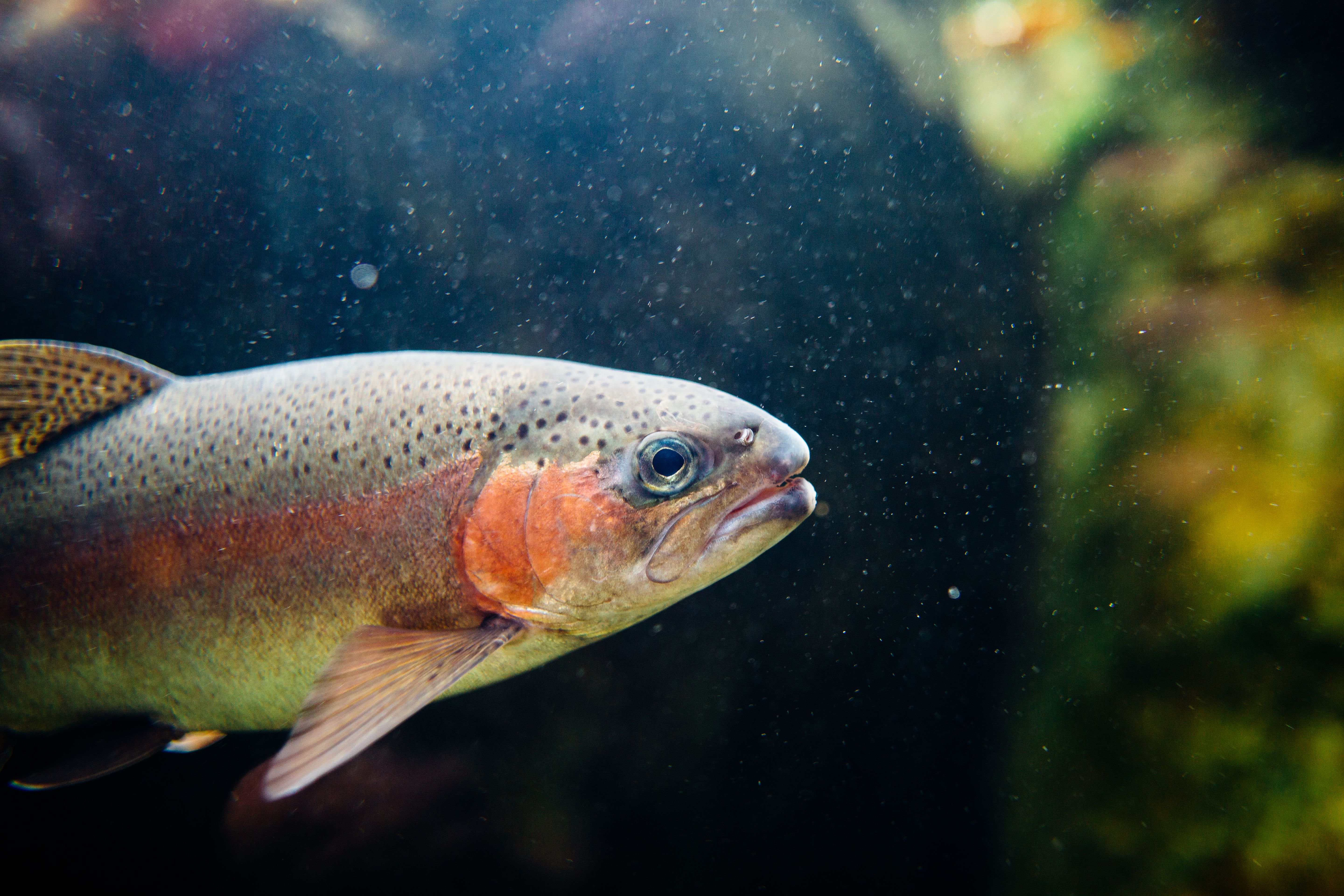
Arctic char (Salvelinus alpinus) is a cold-preferring salmonid with a circumpolar range in Arctic and sub-Arctic fresh waters - and in some stocks also in brackish water. In the Nordics it carries both cultural and commercial weight: wild and farmed char sell as premium fish, often at a higher price per kilo than rainbow trout, thanks to flavour, texture and a "Nordic" market profile.
Farmed Arctic char is a niche next to global salmonids, but it is strategically important in cold inland sites in Sweden, Finland, Iceland, Canada and Alaska. Production uses ponds and raceways with cold spring or lake water, cages in cold lakes, and increasingly land-based systems (semi-flow-through and RAS) where temperature can be held stable year-round.
Compared with rainbow trout, char grows more slowly at the same temperature and tolerates heat less well. Optimal growth often sits in the cooler range (roughly 8-14 °C depending on strain and life stage); above about 16-18 °C stress, reduced feed intake and health risks rise quickly. That makes the species more demanding in warm summers and more dependent on cold intake, shading, deep basins or active cooling in land-based farms.
Water-quality demands are high: stable dissolved oxygen, low ammonia/nitrite, good solids control and gentle hydraulics. Char is sensitive to poor water chemistry and sudden swings - the same filtration, gas and monitoring principles as for other salmonids, but with even less temperature margin.
The premium position means better price but needs consistent quality, traceability and often limited volume. Longer production time and cooling needs raise cost per kg versus trout; profitability depends on differentiating the product (whole fish, fillet, smoking, local/Nordic branding) rather than only chasing lowest production cost. For project developers, char is therefore interesting where cold water is a natural advantage - and where the market pays for the niche.
As with rainbow trout and Atlantic salmon, Arctic char spawning is seasonal if the broodstock environment is not controlled with light and temperature. A farm that wants to sell food fish every month — and fill RAS/semi-flow evenly — cannot rely on a single natural egg pulse. To level the biology you need either frozen milt / planned egg supply and delayed incubation, or control of the broodstock cycle (photoperiod and temperature, several brood groups out of phase), often combined. Otherwise hatchery and grow-out are sized for the peak season and sit partly empty the rest of the year. See Egg incubators (levelling biology over the year).
Char grows more slowly than rainbow trout at the same temperature, but under good cool conditions (~10–12 °C) grow-out is much faster than an overly pessimistic cold-water curve. A useful orientation: about 9 months from ~20 g to ~900 g. Exact time depends on strain, temperature, feed and density — tables are typical ranges, not protocols.
| Stage | Size / weight | Typical duration |
|---|---|---|
| Egg incubation | Fertilised egg → hatch | ~2–3 months (higher °D, cool temp) |
| Alevin / yolk sac | Newly hatched | Weeks to swim-up |
| First-feeding fry | ~0.2–1 g | Weeks–months |
| Fingerling | ~5–50 g | Months |
| Juvenile | ~50–200 g | Months |
| Smaller food fish | ~0.5–0.9 kg | ~15–18 months from egg |
| Typical premium harvest | ~1–1.5 kg | ~18–22 months from egg |
| Large char | ~2–2.5+ kg | ~24–32 months from egg |
Ranges under favourable cool conditions. Heat, density and health lengthen the cycle. Orientation: ~9 months from 20 g to 900 g.
| Time from fertilisation | Approximate size |
|---|---|
| Day 0 | Fertilised egg |
| ~2.5 months | Hatch |
| ~4 months | First feeding |
| ~6.5 months | ~5 g fingerling |
| ~8 months | ~20 g |
| ~12.5 months | ~150 g |
| ~17 months | ~900 g |
| ~19 months | ~1.2 kg |
| ~24 months | ~2 kg |
| ~30 months | ~2.5–3 kg |
Key interval: ~20 g → ~900 g in about 9 months under good cool conditions. Orientation.
Same tool family as for Atlantic salmon and rainbow trout, but with char’s slower growth curve (~8–14 °C) and typical harvest weights. Density, survival, tank classes, growth chart and layout generator included. Orientation — not bankable design.
1. Time from start to target weight
Approximate growth (orientation)
Curve follows char’s slower orientation data; tempo scales the x-axis. Logarithmic weight axis. Orientation — not a feed-control growth model.
2. Production chain toward annual target
H/W = water depth ÷ diameter (round) or flat–flat span (octagon). Optimal default 0.30 ≈ Ø:depth 3.3:1 (typical circular RAS tanks). Lower = flatter/larger footprint; higher = deeper/narrower.
Density (kg/m³) by fish size — adjust to strategy. More stages ⇒ shorter time per tank and sizing to exit weight ⇒ lower total volume.
Stages in the chain
| Stage | Weight (g) | Months | Fish in stage (avg) | Biomass (t) | kg/m³ | Volume (m³) |
|---|
Suggested tank plan
| Tank class | Stage | Days in tank | Unit volume | Depth | Area / tank | Diameter / span | Units | Class volume |
|---|
3. Layout generator (to scale, area = CAPEX) (Experimental)
Packing biased to the golden ratio (φ≈1.618): D+1.0 m cells, grid/shelf and a segment meta-grid so the hall is not one long thin strip.
Packing runs as JS in the browser (grid + shelf). Shared service D+1.0 m. Dashed circle = 0.5 m service zone. Orientation — not construction documentation.
© 2026 DABCE AB
DABCE can help with a review, checklists and short training.
Contact DABCE — contact@dabce.seSee also
Arctic char suits cold inland sites and land-based systems with temperature control. Sources/overview (selection): Nordic/Canadian practice for Salvelinus alpinus; Timmons & Ebeling and others. Growth figures are orientation — strain, temperature, feed and health govern real time. See also FlowFarm.
Sturgeon (Acipenseriformes: Acipenser, Huso and others) are farmed for meat and especially caviar (roe). It is a high-value niche with long generation times, strict traceability and often CITES/species rules. Several species and hybrids are used in aquaculture; Siberian sturgeon (Acipenser baerii) is among the most common in European land-based production.
Unlike salmonids, females take many years to mature — often 5–15+ years depending on species, temperature and feeding. That makes CAPEX, broodstock planning and cash flow critical: caviar revenue comes late, while meat from males and juveniles can bring earlier turnover. Premium niche projects (roe/caviar) therefore need long-term financing and a clear product strategy.
| Species | ♀ maturity (culture) | Comment |
|---|---|---|
| Siberian (A. baerii) | ~6–9 år | Most common in European RAS/raceway |
| Russian (A. gueldenstaedtii) | ~8–14 år | Osietra type; longer cycle |
| Sterlet (A. ruthenus) | ~4–7 år | Smaller fish, earlier roe |
| White (A. transmontanus) | ~8–12 år | Large body; N. America/Europe |
| Beluga (Huso huso) | ~15–20+ år | Very late; highest premium |
| Adriatic (A. naccarii) | ~8–12 år | Mediterranean / hybrid projects |
| Hybrid (e.g. bester) | ~6–10 år | Often chosen for faster production |
Age to first caviar is site-, temperature- and strain-dependent. Orientation — not a breeding protocol.
Water quality: good DO, controlled ammonia/nitrite, low solids load and gentle handling. Sturgeon are benthic and sensitive to poor tank hygiene and grading stress. Sexing (ultrasound) and individual tagging are standard in serious caviar production.
Caviar yield is often stated as a share of female body weight (orientation typically about 8–15% depending on species, condition and processing). Not all egg mass becomes saleable caviar — process yield, grading and market requirements differ. CITES, species labelling and chain documentation are central; farmed caviar must be distinguishable from wild-caught.
After first spawning many females do not spawn every year — intervals of 1–3 years are common. Size the broodstock against the share that is “ready” in a given year, not against 100% of mature females yielding caviar annually.
Pick sturgeon species (preset), number of mature females and average weight. The tool estimates caviar (kg/year), egg numbers for hatchery use and approximate male needs. Orientation — not a caviar plant or CITES application.
© 2026 DABCE AB
DABCE can help with a review, checklists and short training.
Contact DABCE — contact@dabce.seSee also
Sources/overview (selection): established sturgeon/caviar practice (baerii, ruthenus, hybrids); FAO and industry overviews on cultured Acipenseriformes; CITES trade rules. Caviar %, eggs/kg and spawn interval are orientation — species, age, condition and process govern real yield.
Tilapia is the common name for several cichlids in the family Cichlidae; Nile tilapia (Oreochromis niloticus) and related Oreochromis species (and hybrids) dominate world production. It is one of the most farmed fish groups globally — robust, fast-growing in warm water, omnivorous and backed by a mature feed chain. Volume is largest in Asia, Africa and Latin America; in cold Nordic inland sites heating or indoor RAS is required for the species to be relevant.
Historically tilapia ranks among the world’s oldest farmed fishes: in ancient Egypt Nile tilapia appears in art and hieroglyphs, and pond culture along the Nile goes back thousands of years. In modern times selection, monosex (often male) production and intensification in ponds, cages and RAS have made tilapia a staple protein species in many countries — closer to chicken as “volume protein” than to a premium niche.
Tilapia is a warm-water species. Optimal growth typically sits around 28–32 °C; below about 20–22 °C growth slows sharply and below about 12–15 °C mortality risk rises. That is why Nordic outdoor projects without heat are rarely realistic, while heated RAS, greenhouse ponds or tropical sites work. Some strains tolerate a wide salinity range (fresh to brackish), opening coastal areas where freshwater is limited.
Reproduction starts early and often — without control it leads to overcrowding and small fish in ponds. Male monosex (genetic YY, hormone-treated juveniles where allowed, or hybrid systems) is therefore standard in intensive production. Mouthbrooding (the female broods eggs in the mouth) gives high fry survival but complicates breeding comparisons with salmonids.
In ponds the system often acts as an ecosystem: phytoplankton and natural production complement pelleted feed. In RAS/tanks feed and water quality are more “closed” — DO, TAN, nitrite, CO₂ and solids are managed technically. Tilapia tolerate higher density and more challenging water quality than salmonids, but that is no excuse for poor husbandry: gill disease, streptococci and poor FCR still hit hard under stress.
As an omnivore tilapia can use more plant-based feeds than salmon, which lowers feed cost and environmental footprint per kg protein in many LCA comparisons. Grower feed protein is often lower than for salmonids (orientation about 28–36% depending on stage). Typical portion fish is about 400–600 g; cycle time from stocking to harvest is often about 4–8 months at good temperature (sometimes faster in the tropics). Several cycles per year are common in warm regions — a key difference from the long single salmonid cycle.
FCR in well-run intensive culture often sits around 1.3–1.8 (lower in tropical ponds with natural production, higher under stress, low temperature or poor feed quality). Fillet yield is lower than for salmonids — typically about 30–35% for skin-on fillet depending on size and trim — which matters when comparing “kg fish” with “kg saleable fillet”.
Exact duration depends on strain (often improved Oreochromis lines), temperature (~28–30 °C favourable), feed, density and whether monosex is used. Tables are typical ranges under favourable conditions — not protocols.
| Stage | Size / weight | Typical duration |
|---|---|---|
| Egg / mouthbrood | Egg → free-swimming fry | Days–weeks (temp-dependent) |
| Fry / nursery | ~0.1–5 g | Weeks |
| Fingerling / stocking | ~5–50 g | 1–3 months |
| Grow-out | ~50–300 g | Months |
| Portion fish | ~400–600 g | ~4–8 months from stocking |
| Larger food fish | ~0.8–1.2+ kg | Longer cycle / premium |
Ranges under favourable temperature. Strain, monosex, feed and health govern real time.
| Time from stocking (~20 g) | Approximate size (warm water) |
|---|---|
| Month 0 | ~15–30 g fingerling |
| ~2 months | ~80–150 g |
| ~4 months | ~250–400 g |
| ~5–6 months | ~400–550 g portion |
| ~7–8 months | ~550–700 g (temperate/RAS) |
| ~10+ months | ~0.8–1+ kg |
Rule of thumb: ~0.5 kg often about 5–7 months from ~20 g at 28–30 °C. Orientation.
Tilapia tolerate more than salmonids — but DO below about 3–4 mg/L, high nitrite, sudden temperature swings and poor bottom hygiene quickly cause growth stop, gill damage and secondary infections. In ponds, night-time oxygen crashes (after algal blooms) are a classic risk; aeration and contingency are therefore central in intensive pond culture. In RAS the same logic as for other species applies: biofilter, solids removal, gas exchange and alarms.
Important culture health risks include among others streptococci (Streptococcus spp.), Francisella, columnaris and parasites — regionally variable. Biosecurity at stocking, water intake and visitors matters even for “hardy” species. Off-flavour (MIB/geosmin) from cyanobacteria or biofilm can make fish unsaleable until depurated in clean water — a practical cost and logistics issue before harvest.
Globally tilapia is a volume product with price competition. In Europe much frozen fillet is imported; fresh local culture in heated RAS can reach niche prices but must carry the energy cost. In a Nordic climate tilapia is therefore mainly relevant as a comparison species, heated indoor/RAS concept or technology example (water treatment, oxygen, monitoring) — not as a cold-water outdoor species without heat.
In tropical and subtropical countries tilapia is often staple protein with a short cycle, local feed chains and a low technical threshold in ponds — while intensification (biofloc, RAS, cages) is rising. Technology export and advice on water quality, oxygen and monitoring are therefore relevant even when the species itself is not farmed in the Nordics.
The tool estimates fish numbers, standing biomass and volume or pond area from target production (tonnes/year), harvest weight, cycle length, survival and density. Switch between tank/RAS (kg/m³) and pond (kg/ha). Pick a climate preset for typical cycle times and densities. Orientation — not bankable facility design.
© 2026 DABCE AB
DABCE can help with a review, checklists and short training.
Contact DABCE — contact@dabce.seSee also
Sources/overview (selection): FAO on Oreochromis production; WorldFish and NACA on tilapia in Asia/Africa; Timmons & Ebeling (RAS principles); history Rogers 2024 / Costa-Pierce on early Egypt. Density, cycle time and FCR are orientation — climate, strain and husbandry govern real production.
“Catfish” in farming is not one species but several families with similar use: hardy warm-water fish in ponds, tanks and RAS. The two industrially most important lines are African catfish (Clarias, especially C. gariepinus and hybrids) and American channel catfish (Ictalurus punctatus). Pangasius (Pangasianodon) is also farmed widely in Asia, and European wels (Silurus glanis) in more niche European projects. Shared traits are often high hardiness, relatively fast growth in warm water and a role as volume protein rather than a premium niche.
Clarias is especially relevant for intensive land-based systems: the species has air-breathing organs and can sustain very high densities when water quality, feed and handling are maintained. Ictalurus dominates the classic US pond industry with large volume and mature logistics. In a Nordic and European context Clarias is the usual “catfish” reference in heated RAS — while channel catfish is mainly a comparison and pond reference.
| Species / group | Temp (typical) | Systems | Comment |
|---|---|---|---|
| African catfish (C. gariepinus) | ~25–30 °C | Tank, RAS, pond, raceway | Air-breathing; very high density possible |
| Clarias hybrids | ~25–30 °C | Intensive tank/RAS | Often chosen for growth and uniformity |
| Channel catfish (I. punctatus) | ~24–30 °C | Pond (USA), raceway | Large pond industry; classic fillet |
| Pangasius (P. hypophthalmus) | ~26–30 °C | Pond, cage (Asia) | Global volume fillet; own value chain |
| Wels catfish (S. glanis) | ~20–26 °C | Pond, RAS (niche) | Larger fish; European niche |
Temperature and system choice are species- and site-dependent. Orientation — not a culture protocol.
Catfish are warm-water species. For Clarias, fast growth typically sits around 26–30 °C; below about 20–22 °C growth slows and below about 15–17 °C stress and disease risk rise. Channel catfish has a similar warm preference but is often farmed in seasonal ponds where summer drives growth. Air-breathing in Clarias means the species can cope with lower water DO than salmonids — but that is no excuse to run hypoxic: growth, feed conversion and gill health still suffer, and air-breathing raises the fish’s energy cost.
Clarias is omnivorous/carnivorous with aggressive feed intake and cannibalism risk in fry and juvenile stages — grading, density and correct feed size are critical. Channel catfish is a more “classic” pond fish with an established feed chain and less cannibalism in grow-out, but sensitive to off-flavour and summer/oxygen crashes in ponds.
In intensive Clarias tanks, densities often sit far above salmonids (tens to hundreds of kg/m³ depending on oxygen, surface air access, treatment and fish size). Design to real hydraulics and gas exchange — not to “record figures”. In ponds density is more often tonnes per hectare, with aeration as the bottleneck in intensive operation.
Clarias often takes relatively high-protein grower feeds (orientation about 30–40%+ depending on stage) but can use more animal and plant raw materials than salmon. FCR in well-run intensive culture often sits around 1.0–1.5. Channel catfish has a mature US feed industry with typically lower protein than carnivorous salmonids and FCR often around 1.5–2.0 in ponds depending on natural production and season.
Typical harvest weight for Clarias often sits around 0.8–1.5 kg (sometimes larger); channel catfish fillet industry often runs about 0.5–1+ kg depending on market. Cycle time from stocking to harvest is often about 4–8 months in warm water — several cycles per year are realistic in the tropics and in heated RAS.
Exact duration depends on species (Clarias vs Ictalurus), strain/hybrid, temperature, feed and density. Tables below are mainly Clarias-oriented under good warm conditions — not protocols.
| Stage | Size / weight | Typical duration |
|---|---|---|
| Egg incubation | Fertilised egg → hatch | ~1–2 days at ~28 °C (Clarias) |
| Larva / first feed | mg–grams | Weeks; demanding phase |
| Fry / nursery | ~1–10 g | Weeks; grading important |
| Fingerling / stocking | ~10–50 g | 1–3 months |
| Grow-out | ~50–500 g | Months |
| Food fish | ~0.8–1.5 kg | ~4–8 months from stocking |
Ranges under favourable temperature. Cannibalism and grading govern real survival more than in tilapia.
| Time from stocking (~15–20 g) | Approximate size (Clarias, warm) |
|---|---|
| Month 0 | ~15–25 g fingerling |
| ~2 months | ~100–200 g |
| ~4 months | ~400–700 g |
| ~5–6 months | ~0.8–1.2 kg |
| ~7–8 months | ~1.2–1.5+ kg (temperate/RAS) |
Rule of thumb: ~1 kg often about 5–7 months from ~20 g at 26–30 °C. Orientation.
Clarias tolerate more solids and lower DO than salmonids, but nitrite, high TAN at high pH, poor bottom hygiene and abrupt cooling still cause growth stop and disease. In tank/RAS, solids removal, biofilter and gas exchange are bottlenecks at high density — even when the fish “cope” with murkier water. Ensure free surface access for air-breathing in Clarias systems.
Health risks include among others bacterial infections (e.g. Aeromonas, Edwardsiella), parasites and viruses — regionally variable. Cannibalism and grading injuries are practical loss sources. In ponds (especially channel catfish), off-flavour (MIB/geosmin) and summer oxygen crashes are classic market and operational risks. Biosecurity at stocking and water intake matters even for “hardy” species.
Globally catfish is volume protein: channel catfish in the USA, pangasius fillet from Asia, Clarias in Africa and growing intensive systems in Europe/Asia. In Europe Clarias is often sold as fresh or processed product in regional chains; price competition with imported fillet is real. Heated RAS in the Nordics must carry the energy cost — the species is therefore mainly a comparison, technology export (water treatment, oxygen, monitoring) or heated concepts, not a cold outdoor species without heat.
The tool estimates fish numbers, standing biomass and volume or pond area from target production (tonnes/year), harvest weight, cycle length, survival and density. Switch between tank/RAS (kg/m³) and pond (kg/ha). Climate/intensity presets are Clarias-oriented; adjust density for channel catfish ponds. Orientation — not bankable facility design.
© 2026 DABCE AB
DABCE can help with a review, checklists and short training.
Contact DABCE — contact@dabce.seSee also
Sources/overview (selection): FAO and regional practice for Clarias and Ictalurus; European intensive Clarias RAS; USDA/university material on channel catfish ponds; Timmons & Ebeling (RAS principles). Density, cycle time and FCR are orientation — species, climate, strain and husbandry govern real production.
Pikeperch (Sander lucioperca; Eng. pikeperch or zander) is one of Europe’s most valuable freshwater fishes and is regarded as one of the most promising species for diversifying European aquaculture. It is valued for firm, relatively bone-light and mild flesh, which gives a high market value compared with many other freshwater species. Interest in pikeperch farming has grown strongly in Europe, especially in recirculating aquaculture systems (RAS), where production can be controlled year-round.
Unlike established volume species such as salmon, rainbow trout and tilapia, pikeperch is often seen as a premium product with strong willingness to pay in the restaurant and fresh-fish market. It has a shorter industrial farming history than many other commercial fish species, but market demand continues to rise while wild catches in Europe have declined.
The greatest challenge in pikeperch culture is the fry and larval phase. Early feeding is critical and the species is sensitive to stress, unsuitable light regimes and uneven growth. Cannibalism can occur among fry, which requires regular size grading. Low survival and deformities during the larval stage have long been among the main bottlenecks for commercial production.
Many farms therefore choose to buy fingerlings from specialised fry producers or to run separate nursery units before fish are moved to grow-out facilities. Producing the full chain from eggs to market size requires substantially more biological competence and carries higher risk than focusing on grow-out alone.
Once pikeperch has passed the early fry phase it is well suited to intensive production. RAS often uses relatively warm temperatures to maximise growth, while high water quality, good oxygenation and gentle handling remain important because the species is stress-sensitive. Pikeperch can be farmed at relatively high densities and is therefore suited to commercial land-based production.
Besides pure RAS production, pikeperch is farmed extensively in traditional pond systems, especially in Central Europe. Many producers combine pond culture for fry production with RAS for intensive grow-out. The combination can reduce production costs while giving better control of quality, growth and delivery reliability in the later production phase.
| Parameter | Typical range |
|---|---|
| Temperature | 20–28 °C |
| Optimal temperature | 24–26 °C |
| pH | 7,0–8,5 |
| Dissolved oxygen (DO) | >6 mg/L |
| RAS density | Up to about 80–100 kg/m³ |
| Harvest weight | 0,6–3,0 kg |
| Time to about 1 kg | About 15–18 months |
| Production systems | RAS, pond or combined systems |
The values above are general guidelines. Actual performance depends on strain, feed, health status, temperature, water quality and production strategy.
Exact growth rate varies with temperature, feeding, genetic background, light management and culture conditions. The table below shows typical development stages in commercial production. The production sizer below counts from stocking (fingerling) to harvest.
| Stage | Size |
|---|---|
| Larva / first feed | mg–grams |
| Fry / nursery | ~1–10 g |
| Fingerling | 10–50 g |
| Grow-out | 50–600 g |
| Market fish | 0,6–1,5 kg |
| Larger premium fish | 1,5–3,0 kg |
A full production cycle from hatch to about 1 kg market size is often stated as roughly 15–18 months under good production conditions.
Pikeperch is today an established premium species on the European market with strong demand from restaurants, retail and the fresh-fish segment. It is produced commercially in several European countries and is widely seen as an important candidate for further development of sustainable land-based aquaculture. The combination of high market value, good fillet quality and suitability for intensive RAS culture continues to drive investment in the species.
The pikeperch production sizer estimates fish numbers, standing biomass, tank volume or pond area from target production, harvest weight, cycle time, survival and density. The tool is intended as an orientation calculation for concept development and early project work. Results do not replace detailed biological, technical or economic facility design.
© 2026 DABCE AB
DABCE can help with a review, checklists and short training.
Contact DABCE — contact@dabce.seSee also
Sources/overview (selection): Diversify Project — Pikeperch (Sander lucioperca) in European Aquaculture; European Commission Commercial Fish Names — Sander lucioperca; Nguinkal et al. (2019), The First Highly Contiguous Genome Assembly of Pikeperch (Sander lucioperca), an Emerging Aquaculture Species in Europe. Density, cycle time and other figures are orientation — strain, temperature, light and fry management govern real production.
European perch (Perca fluviatilis) is one of Europe’s best-known freshwater fishes and attracts interest for sport fishing, food and aquaculture. It is valued for firm, mild flesh and is a recurring premium product in regional fresh-fish and restaurant markets. Compared with salmonids (salmon, rainbow trout) and tropical volume species, the industrial farming scale is still smaller, but interest in intensification — especially in RAS — has grown in Central Europe and the Nordics.
Perch belongs to the same family as pikeperch (Percidae). Many challenges are therefore similar: a demanding larval phase, cannibalism risk in fry, stress sensitivity and the need for stable water quality. Market size varies regionally — from smaller portions to fillet fish around 200–1000+ g. That affects cycle time, density and economics.
For European perch (Perca fluviatilis), the larval and fry phase is usually the greatest biological and technical challenge in the whole production chain. Although the species grows well in modern RAS and has an attractive market value, commercial expansion is often limited by the difficulty of producing large volumes of high-quality fingerlings.
Perch fry are very small at hatch and have limited energy reserves. Early and correct feeding is therefore critical. Many culture systems use live feed, for example rotifers and Artemia, before fry are gradually weaned onto dry feed. Failed weaning can lead to high mortality and uneven growth.
Fry are also sensitive to light conditions, water quality, handling and sudden environmental changes. Stress in the first weeks can affect both survival and later growth performance. Stable temperature, good water hygiene and steady operating conditions are therefore especially important in this period.
One of the largest problems is the strong size variation that appears early in rearing. Fast-growing individuals can quickly become much larger than their siblings, leading to aggressive behaviour and cannibalism. Regular size grading and close monitoring of the population are required to limit losses. Without effective grading, substantial parts of a year-class can be lost.
Historically, relatively low survival in the larval and fry phase has made it hard to scale production from eggs to harvest fish. Although techniques have improved over recent decades, fingerling production is still a specialised activity that needs high biological competence, established routines and experienced staff.
For this reason many commercial producers choose to buy fry or fingerlings from specialised hatcheries instead of owning the full production chain themselves. A common strategy is to run a separate nursery phase up to a robust fingerling size before fish are moved to the grow-out system. This reduces biological risk and simplifies production.
For new projects and investors it is therefore often more realistic to focus on the grow-out phase and secure fry supply through external suppliers. Establishing full production from eggs to market-ready fish can create more value in the long run, but also means substantially greater technical complexity, higher capital need and greater biological risk.
For most new RAS projects, access to high-quality fingerlings is a more important success factor than the grow-out technology itself. A secure and predictable fry supply is often the real bottleneck for commercial expansion of perch production.
Once perch has passed the fry phase it is suited to intensive grow-out in controlled systems. Optimal growth is often stated around 22–24 °C — somewhat cooler than many pikeperch RAS targets. High DO, good solids handling and gentle handling are important. In comparative trials RAS has often given better survival, FCR and weight uniformity than cages, partly through better control of temperature and light-managed reproduction.
Industrial scale is still smaller than for salmonids. That means fewer “turnkey” references, more site-specific solutions and often a greater need for local market knowledge. At the same time the smaller scale and premium profile make the species interesting for regional land-based projects.
| Parameter | Typical range |
|---|---|
| Temperature | 18–25 °C |
| Optimal temperature | 22–24 °C |
| pH | 7,0–8,5 |
| Dissolved oxygen (DO) | >6 mg/L |
| RAS density | Often about 30–60 kg/m³ (orientation) |
| Harvest weight | 0.2–1+ kg (depending on market) |
| Time to market size | Strongly dependent on target size and temp (orientation) |
| Production systems | RAS, pond or combination |
The values above are general guidelines. Actual performance depends on strain, feed, health status, temperature, light, water quality and production strategy.
Exact growth rate varies with temperature, feeding, genetic background, light management and culture conditions. The table follows the usual chain hatchery → nursery → grow-out. The production sizer below counts from stocking (fingerling) to harvest — not larval survival.
| Stage | Size |
|---|---|
| Hatchery: egg → larva | mg–grams |
| Nursery: larva → fingerling | 1–20 g |
| Fingerling / start grow-out | 1–20 g |
| Grow-out | 20 g → market size |
| Market fish | 200–1000+ g (depending on market) |
Many new projects buy fingerlings and focus on grow-out. A full chain from eggs increases value creation but also risk and complexity.
Perch is sold as fresh fish, fillet and in regional specialty segments. Price per kilo can be high compared with volume species, but the smaller industrial scale also means limited and uneven supply. Farmed perch competes with wild catch and with other percids (e.g. pikeperch). Strong local demand and traceable land-based production are therefore important arguments in concepts and sales.
The perch production sizer estimates fish numbers, standing biomass, tank volume or pond area from target production, harvest weight, cycle time, survival and density. The tool is intended as an orientation calculation for concept development and early project work. Results do not replace detailed biological, technical or economic facility design.
© 2026 DABCE AB
DABCE can help with a review, checklists and short training.
Contact DABCE — contact@dabce.seSee also
Sources/overview (selection): Fontaine et al. on domestication and RAS for Perca fluviatilis; European percid culture (France, Switzerland, Belgium, Central Europe); cage vs RAS comparisons; Diversify and industry overviews on European percids. Density, cycle time and other figures are orientation — strain, temperature, light and fry management govern real production.
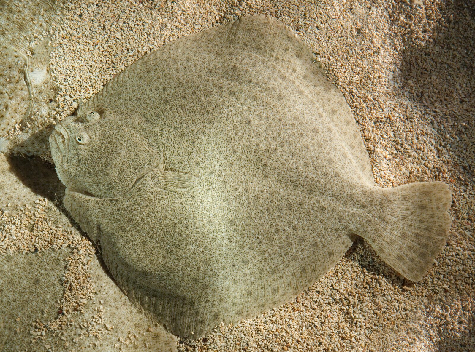
Turbot (Scophthalmus maximus) is a high-value marine flatfish naturally found in the Northeast Atlantic, the Baltic Sea and the North Sea. It is well known in gastronomy and valued for firm white flesh and a high market price. Commercial farming takes place mainly in Europe, using both coastal flow-through systems and modern land-based recirculating aquaculture systems (RAS).
Turbot suits land-based culture because it lives on the bottom and can be held at relatively high biomass densities in shallow tanks. Its flat body shape means tank bottom area is often more important than tank volume when sizing the system. Good water quality, stable temperature and high dissolved oxygen are decisive for optimal growth and fish health.
The greatest challenge in turbot farming is larval production. Larvae are very small and need advanced rearing with live feeds such as rotifers and Artemia before weaning onto dry feed. Metamorphosis from a symmetrical larva to a flatfish, with one eye migrating to the opposite side of the head, is a biologically complex process sensitive to nutritional deficiencies and culture conditions. The larval and fry phase therefore needs high competence and specialised equipment.
As with many marine fish species, larval production is the most technically demanding part of the chain. Commercial success often depends on the ability to produce large volumes of robust fingerlings of even quality. Many commercial producers therefore buy juveniles from specialised hatcheries instead of running full-scale reproduction and larval rearing themselves. For new projects, access to high-quality juveniles is often a more important success factor than the grow-out technology itself.
| Parameter | Typical range |
|---|---|
| Water | Seawater or brackish water |
| Temperature | 14–20 °C |
| Dissolved oxygen (DO) | High and stable |
| Tank type | Shallow round or rectangular tanks with large bottom area |
| Density (orientation) | Often tens of kg/m² bottom area (size-dependent) |
| Systems | Flow-through or RAS |
| Harvest weight | 1–3 kg |
Values are general guidelines. Actual performance depends on strain, feed, salinity, temperature, water quality and production strategy.
Turbot is usually sold at weights between 1 and 3 kg depending on market. Growth time varies with temperature, feeding and production strategy, but production to market size normally takes several years and needs long-term planning of facility capacity. The production sizer below counts from stocking (juveniles) to harvest and sizes mainly bottom area (kg/m²), not volume as for roundfish.
| Stage | Size / note |
|---|---|
| Larva / first feed | Very small; live feed |
| Metamorphosis | Sensitive phase; eye migration |
| Juvenile / stocking | Grams–tens of grams (supplier-dependent) |
| Grow-out | Months–years in shallow tanks |
| Market fish | 1–3 kg |
Long cycle → fewer cycles per year and more standing biomass per tonne of annual production than in fast-growing warm-water species.
Turbot is an established premium species in European gastronomy and export. Farmed turbot complements limited wild catch and can be delivered more evenly through the year from land-based facilities. A high price per kilo must be weighed against the long cycle, marine infrastructure and juvenile supply.
The turbot production sizer estimates fish numbers, standing biomass and required tank bottom area (m²) from target production, harvest weight, cycle time, survival and density in kg/m². Optional water depth gives an orientation tank volume. The tool is an orientation calculation for concept development — not detailed facility design.
© 2026 DABCE AB
DABCE can help with a review, checklists and short training.
Contact DABCE — contact@dabce.seSee also
Sources/overview (selection): European turbot culture (flow-through and RAS); Person-Le Ruyet et al. on growth and density; FAO and industry overviews on Scophthalmus maximus; studies on bottom-area density (kg/m²). Density, cycle time and other figures are orientation — strain, temperature, salinity and juvenile quality govern real production.
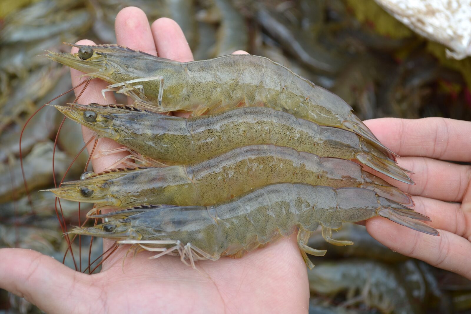
Shrimp (Litopenaeus spp., Penaeus spp. and other farmed shrimp) is the world’s largest aquaculture product by trade value and one of the most important protein sources from aquaculture globally. The dominant farmed species is whiteleg shrimp (Litopenaeus vannamei), which accounts for most of international production. Traditionally shrimp are farmed in earthen ponds and coastal systems in tropical regions, but in recent years intensive biofloc culture and land-based recirculating systems (RAS) have gained commercial interest.
Land-based shrimp farms offer high biosecurity, reduced pathogen spread and the chance to produce fresh premium shrimp near consumer markets in Europe and North America. Technology has made it possible to farm tropical shrimp even in cold climates, but energy costs for heating and water treatment remain an important challenge.
| Species | Comment |
|---|---|
| Whiteleg shrimp (Litopenaeus vannamei) | The world’s most important farmed shrimp. Fast-growing, hardy and relatively adaptable to different salinities. |
| Black tiger shrimp (Penaeus monodon) | Larger species, often premium. High market recognition but generally somewhat slower growth and higher demands than vannamei. |
| Giant river prawn (Macrobrachium rosenbergii) | Farmed mainly in tropical freshwater systems. Large sizes and a different production setup than marine penaeids. |
The production sizer below is mainly oriented toward L. vannamei grow-out.
Shrimp are poikilothermic and growth is strongly driven by water temperature. Temperature control is one of the main cost factors in land-based production in northern Europe.
| Parameter (L. vannamei) | Typical range |
|---|---|
| Optimal | 27–32 °C |
| Acceptable | 24–34 °C |
| Growth declines | Below about 24 °C |
| Mortality risk | Prolonged below about 20 °C |
Orientation — strain, stage and oxygen affect real tolerance.
A major advantage of L. vannamei is its euryhaline nature: the species can be farmed across a wide salinity range. Optimal salinity often sits around 10–30 ppt; culture can go toward nearly freshwater and also full seawater (~35 ppt). At low salinities ion balance becomes critical — sodium, potassium, calcium and magnesium for osmoregulation, shell formation and growth. Many low-salt systems therefore need mineral supplementation.
Biofloc technology is one of the main innovations in modern shrimp farming. Adding a carbon source (e.g. molasses or starch) stimulates bacterial growth that converts ammonium into microbial biomass. Small flocs (biofloc) are kept suspended by intensive aeration and can be grazed by the shrimp.
Biofloc is used across much of the tropical shrimp industry and is often seen as an alternative or complement to classic RAS technology.
Recirculating systems enable production with very low water intake and high biosecurity. Typical components: culture tanks, solids filtration, biological treatment, CO₂ stripping, UV or ozone, oxygenation and temperature control. Advantages are especially large where land, water or biosecurity limit traditional pond culture. See also fry tanks for differences between fish and shrimp tanks (bottom area, substrate, moulting).
| System | Typical density |
|---|---|
| Extensive pond | 0,5–2 kg/m³ |
| Intensive pond | 2–10 kg/m³ |
| Biofloc | 10–30+ kg/m³ |
| Modern RAS | 15–50+ kg/m³ |
Maximum density is often limited by oxygen, biofilter and organic-matter handling. Orientation.
Under optimal conditions L. vannamei can reach market size in a relatively short time. Growth is strongly affected by temperature, feed quality, genetics and water quality.
| From postlarva | Typical time |
|---|---|
| To about 20 g | 3–4 månader |
| To about 30 g | 4–5 månader |
| To about 40 g | 5–6 månader |
Orientation under good temperature. The production sizer counts from stocking (PL/juvenile) to harvest.
Historically disease has been the largest economic risk in shrimp production. Important examples: White Spot Syndrome Virus (WSSV), EMS/AHPND (Early Mortality Syndrome), IMNV (Infectious Myonecrosis Virus) and EHP (Enterocytozoon hepatopenaei). Many modern RAS projects exist specifically to reduce that risk through controlled water supply and strict biosecurity.
Demand is global — from low-cost production in tropical ponds to premium segments with locally produced fresh shrimp. Drivers for European RAS production include shorter supply chains, higher freshness, reduced antibiotic use, better traceability and lower environmental impact. Despite higher production costs, locally produced premium shrimp can often sell at substantially higher prices than imported frozen products.
For land-based shrimp farms, temperature control, oxygenation and biofilter capacity are normally the three most important sizing factors.
The production sizer estimates numbers, standing biomass and culture volume from target production, harvest weight, cycle time, survival and density (kg/m³). Pick a system preset for typical densities and cycle times (L. vannamei-oriented). Orientation for concept development — not bankable facility design.
© 2026 DABCE AB
DABCE can help with a review, checklists and short training.
Contact DABCE — contact@dabce.seSee also
Sources/overview (selection): FAO and industry statistics on Litopenaeus vannamei / Penaeus monodon; biofloc literature (e.g. Avnimelech); RAS and biosecurity overviews for land-based shrimp; WSSV/AHPND/EHP reviews. Density, cycle time and FCR are orientation — strain, temperature, salinity and health govern real production.
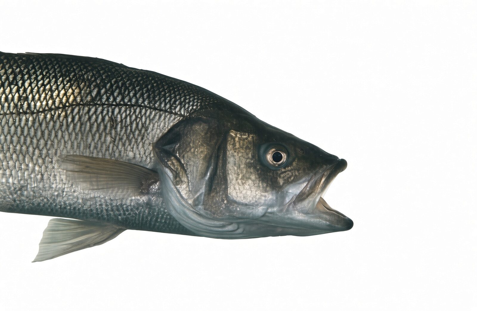
European sea bass (Dicentrarchus labrax) is one of the Mediterranean’s most important farmed fish species and has for decades been a cornerstone of European marine aquaculture. It is farmed mainly in Greece, Turkey, Spain, Italy and Croatia, traditionally in sea cages but increasingly also in land-based recirculating systems (RAS). High market demand, established feed programmes and good adaptability make sea bass an attractive species for modern mariculture.
Sea bass occurs naturally along Europe’s Atlantic coast and in the Mediterranean and Black Sea. It is a predator that feeds on smaller fish, crustaceans and other marine organisms. The fish is euryhaline and can tolerate large salinity variation, so it can be farmed in both marine and brackish waters.
| Parameter | Typical range |
|---|---|
| Optimal | 20–26 °C |
| Acceptable | 12–30 °C |
| Growth declines | Clearly below about 15 °C |
| Stress risk | Prolonged above about 30 °C |
In northern Europe heating is often needed for maximum growth in land-based farms. Orientation.
The most common production form globally. Advantages: low capital cost, natural water exchange and proven technology. Disadvantages: exposure to disease and parasites, risk of storm damage and escapes, and limited control of environmental conditions.
Land-based sea bass production is growing. Advantages: full control of temperature and water quality, high biosecurity, less environmental impact on coastal waters and production closer to consumer markets. Disadvantages: higher capital cost, higher energy use and more advanced operation.
Sea bass has a moderate growth rate compared with many salmonids. Growth is strongly affected by temperature and feeding strategy.
| Stage | Typical time |
|---|---|
| Larva → about 2 g | 2–3 månader |
| 2 g → about 100 g | 5–7 månader |
| 100 g → 400–500 g market weight | 10–16 månader |
| Total production cycle | About 18–24 months |
Orientation under favourable conditions. The production sizer counts from stocking (juvenile) to harvest.
Typical growth curve (orientation)
Solid line = typical growth. Grey dotted lines = faster (earlier + higher weight) and slower (later + lower weight) — bands diverge over time. Log weight axis. Orientation — not a feed-control model.
The most technically advanced part is often the hatchery and fry phase: egg incubation, larval rearing with live feeds (rotifers, Artemia) and gradual weaning onto dry feed. Fry production is today well developed and commercially established across much of the Mediterranean — many grow-out projects therefore buy juveniles.
RAS is increasingly used to reduce infection risk and improve control of the production environment.
Sea bass is an established premium fish on the European market and appears in restaurants, fish counters and retail. The product is sold mainly as whole fresh fish, boneless fillets and chilled premium products. The market benefits from high consumer acceptance, established logistics, stable demand in Europe and good willingness to pay for fresh products.
Sea bass is today regarded as one of the most mature marine species for land-based culture. Strong market demand, well-established fry production and relatively well-known culture parameters make it one of the leading candidates for marine RAS production in Europe.
The production sizer estimates fish numbers, standing biomass and tank volume from target production, harvest weight, cycle time from stocking, survival and density (kg/m³). Presets are grow-out-oriented (juvenile → market). Orientation for concept development — not bankable facility design.
© 2026 DABCE AB
DABCE can help with a review, checklists and short training.
Contact DABCE — contact@dabce.seSee also
Sources/overview (selection): European Mediterranean culture of Dicentrarchus labrax (cages and RAS); FAO and industry statistics; established feed and fry practice in Greece, Turkey, Spain and others. Density, cycle time and FCR are orientation — strain, temperature, salinity and health govern real production.
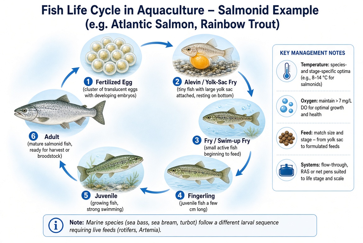
Understanding the fish life cycle is fundamental in aquaculture because each stage has different requirements for water quality, feeding, tank design and management. Hatcheries, nurseries and grow-out systems are often designed around these biological milestones.
| Stage | Temp / oxygen | Feeding | Handling |
|---|---|---|---|
| Egg | Stable temp; high DO; gentle flow | None | Gentle; disinfection; remove dead eggs |
| Alevin | Critical temp & DO | Yolk sac (no external) | Very sensitive — minimise disturbance |
| Fry | Stable WQ; high DO | First feed; correct particle size | Sensitive; frequent checks |
| Fingerling | DO & density matter | Commercial feed | Transport/stocking possible |
| Juvenile | Peak O₂ & biofilter load | High ration; FCR focus | Grading; density control |
| Adult | Species-dependent targets | Maintenance / brood feed | Harvest or broodstock regime |
Orientation — species, system and life stage govern details. See temperature, dissolved oxygen, egg disinfection and fry tanks.
The life cycle begins with the fertilised egg. During incubation, temperature, oxygen and water flow are carefully controlled to maximise survival and minimise fungal growth.
Common management practices include:
In salmonids, the eyed-egg stage is a major milestone — eggs can often be transported more safely after reaching this stage. See also egg incubators and egg disinfection.
After hatching, the larvae are known as alevins in salmonids. At this stage they often remain on the bottom and rely entirely on their internal yolk sac for nutrition.
The duration of the yolk-sac stage varies greatly between species and temperature conditions.
When the yolk sac is absorbed, the fish swim actively and begin feeding externally. This stage is known as fry or swim-up fry.
Critical factors include:
The first-feeding period is often one of the most critical bottlenecks in hatchery production. See fry and larval tanks.
Fingerlings are juvenile fish large enough for transfer to nursery systems, ongrowing tanks or stocking programmes.
Fingerling size varies by species but commonly ranges from a few grams up to about 50–100 g.
The juvenile stage is generally the fastest growth phase in commercial aquaculture. Management focuses on maximising growth rate, maintaining low FCR, controlling stocking density, providing sufficient oxygenation and managing biofilter loading. Most feed consumption and biomass production occur during this stage.
Adult fish may be harvested as food fish or retained as broodstock for reproduction. Food-fish production typically targets market size, product quality, fillet yield and appearance. Broodstock management focuses on reproductive performance, egg quality and genetics.
Atlantic salmon (Salmo salar) have a unique life cycle involving migration between freshwater and seawater. Typical sequence: egg → alevin → fry → parr → smolt → post-smolt → adult. During smoltification the fish undergo physiological changes that prepare them for seawater — one of the most important phases in salmon production. See Atlantic salmon.
Rainbow trout (Oncorhynchus mykiss) follow a similar early life cycle to salmon but are often raised entirely in freshwater or low-salinity brackish water. Typical sequence: egg → alevin → fry → fingerling → juvenile → adult. No seawater transfer is required in most commercial production systems. See rainbow trout.
Marine fish often have a more complex larval stage than salmonids and generally require live feed. Typical sequence: egg → larva → post-larva → juvenile → adult. First feeding often depends on rotifers, Artemia, microalgae and progressive weaning onto dry feed. Larval rearing is often the most technically demanding and expensive phase. See sea bass and turbot.
Every life stage requires different infrastructure, water quality targets and management practices. A modern hatchery may contain separate systems for egg incubation, fry rearing, nursery production and broodstock management. Understanding the fish life cycle helps operators optimise growth, survival, biosecurity and production economics throughout the entire farming process.
See also
Fish physiology governs how fish respond to water quality, temperature, oxygen levels, salinity and the culture environment. Understanding gills, osmoregulation, metabolism and stress response makes it easier to optimise both fish health and production results.
The gills are the fish’s most important organ for contact with surrounding water. They are responsible not only for respiration but also for salt regulation, acid–base balance and excretion of nitrogenous waste.
The gills are used among other things for:
Because gill tissue is very thin to allow efficient gas exchange, it is also sensitive to environmental disturbance.
When the gills are damaged, oxygen uptake deteriorates, which often leads to reduced growth, poorer FCR and higher disease sensitivity. See also dissolved oxygen, ammonia, nitrite, CO₂ and turbidity/TSS.
Osmoregulation is the fish’s ability to control water and salt balance in the body. It is an energy-demanding process that runs continuously.
Freshwater contains far fewer salts than fish body fluids. Water therefore diffuses into the fish and salts diffuse out; the fish produces large volumes of dilute urine and the gills actively take up ions from the water. Species such as Arctic char, rainbow trout, brown trout and perch use large amounts of energy to maintain salt balance.
In seawater the situation is reversed: the fish loses water to the surroundings, salt diffuses in, the fish drinks seawater and excess ions are pumped out via the gills. Examples include sea bass, sea bream and turbot.
Brackish water sits between fresh and seawater and can in some cases mean lower energy demand for osmoregulation. For several species the right salinity can reduce physiological stress, improve growth, improve feed utilisation and increase survival. See salinity.
Besides salinity, ion composition matters. Important ions include calcium (Ca²⁺), magnesium (Mg²⁺), sodium (Na⁺), potassium (K⁺), chloride (Cl⁻) and bicarbonate (HCO₃⁻). These affect osmoregulation, nerve function, muscle function, skeletal development and egg/embryo development. Very soft waters may therefore need remineralisation for sensitive species or life stages. See mineral and ion management and hardness.
Fish are ectothermic — body temperature follows water temperature. As temperature rises, metabolism, feed ration, oxygen consumption and growth increase up to the species optimum. If temperature becomes too high, stress rises, oxygen demand increases sharply, appetite may fall and mortality may rise. Each species therefore has a specific temperature range where growth is best. See temperature.
Stress is a natural physiological reaction, but prolonged chronic stress is one of the most common causes of production problems in aquaculture.
Many of the economic losses in aquaculture are directly or indirectly linked to chronic stress.
Reproduction is controlled by complex environmental signals. Important factors include photoperiod (day length), temperature, nutrient availability, salinity and hormonal signals. Many farms use programmed lighting to control maturation, spawning periods and growth.
Broodstock often need different environmental conditions than production fish. Typical measures include controlled light programmes, special temperature regimes, specialised feeds, lower stress levels and careful health control. Good broodstock management affects egg quality, fertilisation rate, hatch rate, larval survival and growth of the next generation.
Almost all technical systems on a farm ultimately aim to support fish physiology. Oxygenation, biofilters, temperature control, degassing, UV systems and feeding are about giving the fish optimal conditions for gas exchange, osmoregulation, growth and reproduction. When physiology works well, more energy goes to growth and less to coping with stress, which gives better fish health, higher survival and lower production cost.
See also
Fish, eggs and fry can be affected by fungi, bacteria, viruses and parasites. Risk often rises with stress, high density, poor water quality, oxygen shortage, sharp temperature changes or handling. Many outbreaks do not start with the pathogen itself but with fish first weakened by the environment.
Early signs are often non-specific: reduced appetite, slower growth, rising mortality, increased mucus, darkening, gasping or changed behaviour. Fish that isolate from the group or crowd at inlets, oxygenation points or the surface often signal that something is wrong.
Viral diseases often lack effective treatment. Preventive biosecurity, health control and infection protection are therefore critical.
The following symptoms should always be taken seriously:
The best disease treatment is to avoid outbreaks from the start.
If an outbreak is suspected, isolate the affected group as far as possible. Minimise movement of fish, equipment and staff between departments. Record symptoms, mortality, water quality and recent changes on the site.
Contact a fish health veterinarian or the competent authority if a serious or notifiable disease is suspected. Several viral and parasitic diseases are covered by national and international disease-control rules.
This knowledge page does not replace professional diagnosis, laboratory analysis or veterinary advice.
See also
Biosecurity is often the most cost-effective disease insurance on a fish farm. Many serious outbreaks are not introduced via water or wild fish but through purchases of eggs, fry, juveniles, live feed, equipment or people moving between sites. Once an infection is established it can be very hard and expensive to eliminate. Modern aquaculture therefore aims to prevent pathogen introduction rather than treat after the fact.
Many farmers focus on pathogens but underestimate the importance of feed. Feed directly affects the fish’s immune system, gut health and resistance to infection.
UV is one of the most important biosecurity barriers in modern RAS and flow-through systems.
Ozone is one of the strongest oxidants used in aquaculture. Used correctly it can improve water quality substantially; used incorrectly it can damage fish very quickly.
Seawater requires special caution. Seawater contains high levels of bromide ions (Br⁻). When ozone reacts with bromide, oxidation products form, including hypobromous acid (HOBr) and bromate (BrO₃⁻). These brominated oxidants can be far more persistent than ozone itself.
AOP often combines UV with oxidants such as ozone or hydrogen peroxide. The aim is to form highly reactive hydroxyl radicals (•OH) that can break down substances otherwise hard to remove.
No single measure stops all diseases. Successful biosecurity is built from several independent barriers:
Rule of thumb: Many of aquaculture’s worst disease outbreaks start with a single introduced fish, one egg lot or one piece of equipment. A consistent biosecurity culture is therefore as important as biofilters, oxygenation and water quality for producing healthy fish.
See also
If you need assistance with biosecurity, quarantine or infection barriers, don’t hesitate to contact DABCE.
Contact DABCE — contact@dabce.seHealthy aquatic organisms are the foundation of profitable aquaculture. Good welfare is not only an ethical objective or regulatory requirement. It is closely linked to survival, growth, feed conversion, disease resistance, product quality and overall farm performance.
Poorly managed aquaculture systems can suffer from a wide range of production and commercial problems long before catastrophic disease outbreaks occur. Chronic stress, poor water quality, inadequate nutrition and weak biosecurity often reduce growth, increase mortalities and lower product quality. These losses can directly affect farm profitability and market access.
In severe cases, producers may face:
Modern aquaculture therefore focuses on producing not only more biomass, but also healthier, safer and more consistent products. Good welfare includes among other things enough oxygen, low stress, gentle handling, suitable density and humane slaughter — while certification and law continue to tighten in the EU and the Nordics.
Not all aquaculture products achieve the same market value.
Premium Atlantic salmon produced in well-managed farms with excellent water quality, strong biosecurity, controlled nutrition and careful harvesting often achieves significantly higher market acceptance than lower-grade products showing soft flesh, pigmentation issues, mechanical damage or inconsistent quality.
Similarly, shrimp produced in highly controlled systems may achieve premiums through:
At the other end of the spectrum, poorly managed production systems can experience high variation in survival, growth and product quality. In some regions, extensive pond systems may produce large volumes at low cost, but performance and final quality can vary significantly depending on management practices, water quality, disease pressure and harvesting methods.
The highest-value aquaculture products are typically associated with:
From a farming perspective, welfare can often be viewed as the ability of the cultured organism to allocate energy toward growth and production rather than coping with environmental stress.
A healthy fish, shrimp or lobster uses feed more efficiently, grows more predictably and is generally less susceptible to disease. Conversely, organisms exposed to chronic stress divert energy away from growth, resulting in poorer biological and economic performance.
For most commercial farms, improvements in welfare frequently translate into:
In this sense, welfare is not separate from production. It is one of the key drivers of sustainable and economically successful aquaculture.
See also
If you need assistance with welfare, health or production performance, don’t hesitate to contact DABCE.
Contact DABCE — contact@dabce.seFCR (Feed Conversion Ratio) = kg feed / kg fish gain. It is one of the most important KPIs in aquaculture: it drives feed cost, water quality, sludge production and carbon footprint. Lower FCR means more growth per kilogram of feed — and usually lower OPEX and environmental load.
FCR is not only economics: every kilogram of feed drives TAN, TSS, oxygen demand and sludge. See feed types, feeding systems, ammonia and sludge.
See also
Feed is the single largest operating cost in most aquaculture systems and the primary driver of fish growth, water quality and farm profitability. Modern aquaculture feeds are carefully formulated to provide the correct balance of protein, lipids, carbohydrates, vitamins, minerals and functional ingredients for each species and life stage.
The ideal feed delivers growth and health while minimising waste, FCR and environmental load. Ultimately every kilogram of feed becomes fish biomass, dissolved waste or solid waste (sludge). Feed quality therefore affects both production and water-treatment demand.
See also
Protein is the most important nutritional component. Fish use it to build muscle, organs, skin, enzymes, hormones and immune tissues — both growth and maintenance.
Traditionally, high-quality feeds relied on fish meal and fish-protein concentrates. Modern feeds increasingly use alternatives: soy protein concentrates, wheat gluten, pea protein, insect meal, single-cell proteins, fermentation-derived ingredients and algae-based proteins. The goal is not simply high protein, but the correct balance of essential amino acids.
Protein that is not converted into fish biomass is largely excreted as ammonia (TAN) and loads the biofilter. See Ammonia / TAN and MBBR.
Lipids are the primary energy source in many aquaculture diets. By supplying energy through fats, protein can be retained for growth rather than burned for metabolism. Lipids contribute to energy, growth, feed efficiency, health, product quality and omega-3 content.
High-energy feeds are particularly common in salmonids, where dietary fat can be high (in some grower feeds above 30%). Common sources include fish oil, vegetable oils, algal oils and blends. Higher energy can improve FCR but may also increase fat deposition if growing conditions are not optimal. No recipe percentages here — use the feed analysis and the species target.
Fish generally use carbohydrates less efficiently than terrestrial livestock, although warm-water species often use them better than cold-water carnivores. Carbohydrates may provide energy, pellet structure, feed stability and lower feed cost. Examples include wheat, corn, starches and other cereals. The optimal level varies widely between species.
Vitamins are required in small amounts but are essential. Important ones include A, D, E, K, C and B-complex. Deficiencies can lead to poor growth, skeletal deformities, reduced immunity and higher mortality. Most commercial feeds contain a complete vitamin premix for the species and life stage. No dose in the text.
Fish need minerals for skeleton, osmoregulation, enzymes, reproduction and metabolism. Important ones include calcium, phosphorus, magnesium, potassium, sodium, zinc, selenium and iron. Some can be absorbed from the water; others must come in the feed. The contribution from water chemistry is especially important in freshwater. See hardness, salinity and mineral and ion management.
Some feeds contain pigments that influence flesh colour and market value. The best-known is astaxanthin, which gives salmon and trout the pink–orange colour consumers expect. Without supplementation, salmonid flesh would be much paler. Other species may use different pigment sources depending on the product goal. No doses here.
Modern feeds increasingly contain functional additives beyond basic nutrition: probiotics, prebiotics, immunostimulants, organic acids, specialised amino acids, algal products and yeast extracts. They may support immunity, stress resistance, gut health, feed utilisation and survival. Use continues to grow as producers look for alternatives to antibiotics and other interventions. This is not treatment advice.
Feed is the main source of nutrients entering the system. Higher feeding rates mean more oxygen demand, more ammonia and carbon dioxide, more sludge and a heavier biofilter load. That is why feeding rate often sets the size of biofilters, oxygen systems, drum filters, protein skimmers and sludge handling. In intensive aquaculture, capacity is frequently calculated from maximum feed load rather than biomass alone. See feeding systems, sludge and RAS.
Feed is far more than fish food. It is the primary input that drives growth, water quality, waste, economics and final product quality. A well-formulated feed matched to species, life stage and production goals can improve growth, reduce FCR, support health and increase profitability.
Protein builds fish. Lipids provide energy. Vitamins and minerals keep the biological machinery running. The best feed is not simply the cheapest or the highest-protein feed. It is the feed that produces the most healthy fish biomass while minimising waste and keeping the best possible FCR.
DABCE can help with a review, checklists and short training.
Contact DABCE — contact@dabce.seSources/overview (selection): Timmons & Ebeling; established feed practice for salmonids and warm-water species. Orientation, not a feed recipe or a dose. No prices. See also feeding systems, FCR, Ammonia / TAN and mineral and ion management.
Choosing the correct pellet size is just as important as selecting the correct feed formulation. Pellets that are too large may be difficult to consume. Pellets that are too small can increase losses, reduce feeding efficiency and add unnecessary waste. Manufacturers therefore offer a wide range of sizes for species and life stage.
See also
The table is orientation. Actual size follows species, mouth form and the manufacturer table — do not invent millimetres.
| Fish size | Typical feed form |
|---|---|
| Larvae | Live feed, microdiets (< 0.5 mm) |
| Fry (about 0.1–5 g) | Small starter pellets — manufacturer table |
| Fingerlings (about 5–20 g) | Next step in the manufacturer series |
| Juveniles (about 20–100 g) | Mid size — species and manufacturer |
| Grow-out (about 100–500 g) | Larger pellets — see species notes below |
| Large grow-out (> 500 g) | Largest commercial size for the species |
Not a dosing table. Always use the current feed series.
Different species have different feeding behaviour and mouth structure. That influences optimal pellet size as much as body weight.
Salmonids (salmon, trout, Arctic char) typically use larger pellets as they grow. Commercial grow-out diets often sit in the 4–12 mm range; large harvest salmon may receive pellets above 10 mm. Tilapia generally prefer somewhat smaller pellets at a given body weight; common sizes sit in the 1–6 mm range. Sea bass and sea bream often use 1–8 mm depending on size — buoyancy and sinking also matter. Shrimp use specialised sinking feeds that step up as they grow. Always species + manufacturer, not a generic millimetre rule.
Correct sizing can improve intake, growth, FCR, feeding behaviour and water quality. The wrong size can increase losses, reduce growth, raise FCR and produce more sludge and ammonia. In intensive RAS even small increases in wasted feed load drum filters, protein skimmers, biofilters and sludge handling. See FCR, sludge and Ammonia / TAN.
As fish grow, pellet size is stepped up. An example for trout or salmon (orientation, not a product line): 0.8 mm → 1.5 mm → 2 mm → 3 mm → 4.5 mm → 6 mm → 9 mm → 12 mm. Larger pellets too early reduce growth because smaller fish cannot eat them efficiently. Excessively small pellets to large fish increase losses and feeding time.
Feed composition determines what the fish eat. Pellet size determines how efficiently they can eat it. A good feed in the wrong size can perform worse than a slightly less advanced feed in the right size. As fish grow, pellet size should grow with them.
DABCE can help with a review, checklists and short training.
Contact DABCE — contact@dabce.seSources/overview (selection): established commercial feed practice for salmonids, tilapia and marine fish; manufacturer size tables. Orientation, not a product or dosing table. Empty millimetre cells in the draft were left unfilled on purpose. See also feed types and feeding systems.
Feeding is one of the most important daily operations in aquaculture. Feed typically represents the largest operating cost on a fish farm and directly influences growth, FCR, water quality, fish welfare and profitability. The goal is simple: provide enough feed to maximise growth without wasting feed or overloading the water-treatment system.
Every kilogram of uneaten feed becomes a cost twice: first when purchased and again when it creates additional waste that must be removed.
See also
Feeding influences nearly every aspect of production: growth, FCR, survival, water quality, biofilter loading, oxygen demand, ammonia, sludge and economics. Insufficient feeding limits growth. Excessive feeding wastes money and increases environmental loading.
A useful rule: feed drives growth, but feed also drives waste production.
Hand feeding remains common in hatcheries, broodstock facilities, research systems and smaller farms.
Operators can observe feeding activity, swimming, condition and early disease signs. The drawback is labour, and rations can differ between staff.
Automatic feeders distribute feed on a programmed schedule. Common types include belt, vibratory and screw feeders and pneumatic delivery.
Frequent small meals often improve utilisation compared with a few large daily feedings. That can improve growth and FCR and even out oxygen demand and ammonia production.
Demand feeders release feed when the fish trigger a pendulum or similar mechanism. The fish determine how often a small ration is released. They have been used with species such as rainbow trout, Arctic char, tilapia and carp.
Dominant fish may control access. Stress, stocking density and environmental conditions also affect how fish use the feeder.
Modern farms increasingly use underwater cameras in real time. Operators see feeding intensity, pellet behaviour, fish distribution and when waste begins. Feeding can then be cut before significant losses occur.
Advanced systems use machine vision and AI to follow swimming, feeding response, distribution, pellet consumption and the environment. Feeding is adjusted from observed behaviour, not only from a fixed table. See AI, image analysis and biomass.
Large salmon operations increasingly rely on camera- or AI-assisted feeding. The best system is not always the most advanced — it is the one that consistently delivers the right amount at the right time.
Feed is the primary source of waste in the system. What is not converted into fish becomes sludge, dissolved organics, carbon dioxide, ammonia (TAN) and phosphorus. Overfeeding therefore reduces water quality and raises ammonia, oxygen demand, organic load and sludge. See Ammonia / TAN, dissolved oxygen and sludge.
In RAS the peak daily feed often sets the size of biofilters, oxygen systems, drum filters and sludge handling. That is why many design calculations start from peak feed, not only from biomass. See RAS and MBBR.
The right frequency depends on species, size, temperature and system. Small fish have a higher metabolic rate and usually do better with many meals. The table is orientation, not a recipe.
| Life stage | Typical frequency |
|---|---|
| Larvae | Continuous or many times per day |
| Fry | 8–24 feedings/day |
| Juveniles | 4–12 feedings/day |
| Grow-out | Fewer, larger meals — species, temperature and system decide |
Orientation. Modern automatic systems often spread feed through daylight hours.
How well the system works is often measured as FCR = feed given ÷ biomass produced. Example: 1.0 kg feed → 1.0 kg growth is FCR 1.0; 1.2 kg feed → 1.0 kg growth is FCR 1.2. Reducing waste is one of the fastest ways to improve FCR. See FCR and fish price, energy and risk.
The best feeding system is not necessarily the most advanced. The best system is the one that consistently delivers the right amount at the right time while minimising waste. Whether hand, automatic, demand, camera or AI, the objective is the same: maximise growth, minimise waste, protect water quality and achieve the best possible FCR.
The fish decide how much they can use efficiently. The farmer's challenge is delivering exactly that amount, no more and no less. Every uneaten pellet becomes a water-quality problem. Every efficiently consumed pellet becomes fish biomass.
DABCE can help with a review, checklists and short training.
Contact DABCE — contact@dabce.seSources/overview (selection): Timmons & Ebeling; established hatchery and RAS feeding practice. The frequency table is orientation, not a recipe. No doses or feed prices. See also FCR, sludge and Ammonia / TAN.
Aquaculture sludge is a mixture of solid wastes generated during fish, shrimp and shellfish production. It consists primarily of fish faeces, uneaten feed, feed fines, detached biofilm, bacterial biomass and other suspended organic particles removed from the water-treatment system.
Although sludge is often viewed as a waste product, it actually contains a large share of the nutrients entering the farm through feed: organic carbon, nitrogen, phosphorus, minerals and trace elements. Effective sludge management therefore plays an important role in fish health, biofilter performance, environmental compliance and resource recovery.
See also
Most aquaculture sludge originates from feed. When feed enters a farming system it is ultimately divided into fish biomass (growth), dissolved waste products and solid waste products. The solid fraction becomes sludge.
Feed in
↓
Growth (fish biomass)
+
Dissolved waste (TAN, dissolved P, DOC …)
+
Solid waste → sludge
The solid fraction typically includes:
The amount of sludge produced depends on feed composition, feed digestibility, feeding practices, species, FCR and system design. As production intensity increases, sludge production also increases. See FCR and feeding systems.
If sludge is not removed quickly, bacteria begin breaking down the organic material. This results in increased oxygen demand, higher carbon dioxide production, increased ammonia generation, biofilter overloading, reduced water clarity and increased disease risk.
Fresh faeces and feed particles are generally easier to remove than degraded sludge. Once solids begin breaking down, much of the nutrient load shifts into dissolved forms that are more difficult and expensive to treat. For this reason one of the fundamental principles of aquaculture water treatment is: remove solids early and remove them often.
The exact composition varies between species and feeds, but sludge typically contains organic carbon, nitrogen, phosphorus, calcium, magnesium, trace minerals and water. Because sludge is largely organic matter, it continues to decompose after collection unless it is stabilised or further treated.
Poorly managed storage can produce ammonia, methane, hydrogen sulphide and carbon dioxide.
RAS facilities produce concentrated sludge because most solids are captured before water is reused. Common collection points include drum filters, settling cones, hydrocyclones, protein skimmers and biofilter purge systems. Because the solids are concentrated, sludge handling becomes an important part of overall system design. See RAS, drum filters and protein skimmers.
Flow-through farms generally produce more dilute sludge because a significant portion of solids leaves with the discharged water. Sedimentation basins are often used to capture solids before discharge. See flow-through systems.
Pond systems accumulate sludge on the pond bottom over time: fish waste, feed residues, algae and natural organic matter. Excessive accumulation can reduce water quality and increase oxygen demand. See ponds.
In sea cages, most sludge settles to the seabed beneath the farm. Management therefore focuses on site selection, current velocity, seafloor monitoring and environmental carrying capacity — not on an in-loop filter. See net pens.
One of the most important reasons for sludge removal is protecting biological filtration. When solids enter biofilters they can reduce oxygen transfer, clog media, promote unwanted bacterial growth, reduce nitrification efficiency and increase maintenance. A healthy biofilter relies on effective upstream solids management. A useful rule in RAS design is: the best biofilter is protected by the best solids-removal system. See MBBR, fixed bed and trickling filters.
Aquaculture sludge is the concentrated solid waste stream of a fish farm. It originates primarily from feed and faeces, but it also contains nutrients that can potentially be recovered and reused. Effective sludge management protects fish health, water quality, biofilter performance, receiving waters and farm economics. As aquaculture intensifies, sludge management is increasingly a core part of sustainable farming rather than only a disposal challenge. See collection and nutrient recovery.
Feed enters the farm. Fish become growth. The remaining nutrients become dissolved waste or sludge. The faster solids are removed, the easier it is to protect water quality, maintain biofilter performance and recover valuable nutrients. A simple calculator from production and FCR is under collection and dewatering.
DABCE can help with a review, checklists and short training.
Contact DABCE — contact@dabce.seSources/overview (selection): Timmons & Ebeling, Recirculating Aquaculture; established RAS and receiving-water practice on solids and sludge. Orientation, not permit values or kg sludge per kg feed. See also collection, nutrient recovery, FCR and Ammonia / TAN.
The goal is to capture solids early and concentrate them — remove as much water as possible — so transport, storage and further treatment stay manageable. Fresh particles are easier to remove than degraded sludge. See what aquaculture sludge is.
See also
In RAS the sludge is often already concentrated at drum filters and cones. In flow-through it is more dilute and is often captured in a sedimentation basin before the receiving water. In ponds the material sits on the bottom; in sea cages it settles on the seabed under the farm.
Reducing sludge volume lowers transport cost, storage need and disposal cost. Dewatering does not remove the nutrients — it removes water. Dry-matter content and odour depend on how quickly sludge is handled and whether it is aerated, covered or treated further.
Enter production and FCR. Choose whether there is a biostage (secondary sludge) and optional dewatering. Moisture follows the technology but can be edited. Primary DS is the midpoint of 200–400 g/kg feed from the mass-flow figure — edit if you have a feed analysis.
© 2026 DABCE AB
When solids remain in the loop, oxygen demand, CO₂ and ammonia rise and the biofilter fouls. Upstream solids removal is what protects MBBR, fixed-bed and trickling filters. The best biofilter is protected by the best solids-removal system.
DABCE can help with a review, checklists and short training.
Contact DABCE — contact@dabce.seSources/overview (selection): Timmons & Ebeling; the mass-flow figure 200–400 g TSS/kg feed; established RAS practice on drum filters, settling and dewatering. The calculator is orientation, not a sizing of mesh, geobags or presses.
Modern aquaculture increasingly views sludge as a resource rather than simply a waste stream. Much of the nitrogen and phosphorus entering a farm through feed ultimately leaves in sludge. As nutrient recovery, circular-economy solutions and fertiliser security become more important, that residual stream may gain value — provided storage, treatment, hygiene and rules are managed.
A useful way to think about sludge is concentrated nutrients that were not converted into fish biomass. The challenge is therefore not only disposal, but how those nutrients can be recovered, stabilised and reused.
See also
Every kilogram of feed contains organic carbon, nitrogen, phosphorus, minerals and trace elements. Part becomes fish biomass. The rest leaves as sludge, dissolved waste or carbon dioxide. Historically sludge was often a disposal problem. Farms increasingly ask how nutrients can be recovered and reused rather than lost from the food chain.
Compared with municipal wastewater sludge, industrial sludge or mixed organic streams, aquaculture sludge is often more predictable. It comes almost entirely from faeces, uneaten feed, fines, biofilm and microbial biomass. It generally does not carry road runoff, household chemicals, pharmaceuticals, industrial effluent or the metal load of many municipal sludges. Nutrient content is therefore often easier to characterise, and the material may be more attractive for recovery.
In a simplified sense the sludge largely comes from feed- or food-grade ingredients that entered the farm. That is not a regulatory approval. Water source, species, system, feed and local rules still decide what reuse is allowed. Analysis is always required before land application or product development.
Composting converts organic sludge into a stable soil amendment. Advantages: simple technology, lower volume, organic-matter recovery and possible agricultural use. Suitability depends on rules, sludge quality and available markets.
Because feed carries nitrogen and phosphorus, sludge can in some cases enter fertiliser products. That may require dewatering, stabilisation, hygienisation and nutrient characterisation — depending on the rules. Economic value often depends on transport distance, nutrient concentration and access to farms. For freshwater aquaculture this is often one of the most direct routes. No prices or recipes here.
Besides sludge, farms also discharge or recirculate nutrient-rich water — especially in RAS, semi-flow and low-exchange systems. After solids removal, effluent or recirculated water can contain dissolved nutrients (e.g. nitrate, phosphorus and minerals) that may be used directly or after polishing as fertigation water in agriculture, horticulture and aquaponics. In aquaponics the principle is that dissolved nutrients from the fish drive plant production in the same water loop. In agriculture and horticulture, suitably treated process water can reduce mineral-fertiliser demand while lowering discharge load — provided salinity, hygiene, pathogens, veterinary residues and local rules allow it. Marine or strongly brackish water is often unsuitable for common land crops without desalination or salt-tolerant crops. Orientation — not an irrigation or permit recipe.
Anaerobic digestion converts organic matter into biogas and digestate. Biogas can provide heat, electricity or be upgraded to biomethane. The digestate retains much of the nutrient value and may be used as a fertiliser resource where rules allow.
Co-digestion with manure, food waste or other organics is often considered because pure aquaculture sludge can have relatively low dry-matter content. Digestion also stabilises the sludge and reduces methane that might otherwise form in unmanaged storage.
HTC treats wet biomass at elevated temperature and pressure. Unlike many thermal technologies, HTC can process sludge with a high water content without extensive drying. The process typically produces hydrochar, nutrient-rich process water and small amounts of gas.
For wet aquaculture sludge, HTC is of growing interest because drying cost is often the main barrier to conventional thermal treatment. This is orientation, not a process design.
Phosphorus is a finite and strategically important nutrient for food production. Emerging routes include struvite precipitation, extraction, ash-based recovery and nutrient concentration. As agriculture depends more on recycling, phosphorus from sludge may become attractive even in smaller farms. No process sizing here.
Not all sludge is equal. The right pathway depends on volume, dry-matter content, nutrient concentration, transport distance, energy, markets and rules. Sludge from marine or brackish systems carries dissolved salts that may limit some land-application options. What works for a freshwater trout farm may not suit a marine sea-bass or sea-bream site. The solution is site-specific, not universal. See salinity.
Fresh sludge stays biologically active and keeps decomposing. Without stabilisation, storage may generate ammonia, carbon dioxide, methane and hydrogen sulphide — odour, nutrient losses, greenhouse gases and handling problems. Common routes are composting, digestion, HTC or other biological or thermal treatment.
Good practice includes covered storage, controlled runoff, odour control, leachate management and monitoring of storage conditions. The aim is to keep nutrients while minimising emissions and nuisance. Storage is part of the process — not an afterthought.
Use of aquaculture sludge is regulated in many jurisdictions: storage, transport, land application, hygienisation, nutrient management, animal-by-product classification and environmental permitting. Rules vary widely between countries. This section is an overview only — not a permit guide, legal approval, fertiliser recommendation or product approval.
Sludge carries nutrients from the feed. Unlike many waste streams it is typically rich in organic matter, nitrogen and phosphorus and often freer of the contaminants associated with municipal wastewater sludge and many industrial residues. Whether those nutrients become a disposal cost or a recoverable resource depends on how the sludge is managed. As aquaculture intensifies and society emphasises recycling, carbon management and sustainable food, sludge handling becomes part of the value chain — not only the waste chain.
Feed enters the farm as nutrients. Fish become biomass. The remaining nutrients end up in dissolved wastes or sludge. The faster solids are captured and the better sludge is managed, the greater the chance to recover value through fertiliser, digestion, HTC, phosphorus recovery or other circular pathways. Aquaculture sludge is not just a waste stream. In many cases it is a concentrated nutrient resource waiting to be recovered.
DABCE can help with a review, checklists and short training.
Contact DABCE — contact@dabce.seSources / overview (selection): General engineering practice and published literature on aquaculture sludge management, nutrient recovery, anaerobic digestion, hydrothermal carbonisation (HTC), composting, fertilizer production, phosphorus recovery, circular bioeconomy systems, fish-processing residuals, digestate management and resource recovery from aquatic biomass. Also reflects established approaches used in aquaculture, wastewater, food-processing and organic-residual management sectors. Local regulations governing sludge handling, fertilizers, biosolids, environmental permits, animal by-products, nutrient management and effluent discharge vary between countries and regions. This section provides technical orientation only and should not be interpreted as process design, regulatory guidance, permit advice, fertilizer recommendation, investment advice or product approval. Economics, process performance, recovery efficiencies and product suitability depend on feedstock characteristics, scale, local regulations, markets and project-specific engineering.
See also
Oxygen demand in a farm is driven mainly by biomass, feeding intensity, temperature and species. Fish and the biofilter compete for the same oxygen — especially after peak feeding. Too-low DO causes stress, poorer FCR and in the worst case mortality.
Concept models often use rules of thumb in kg O₂ per kg feed. Real design needs species, temperature, saturation and system hydraulics. See dissolved oxygen and oxygen cones.
See also
Oxygen can be supplied via air (aeration/degassing) or pure oxygen (PSA, LOX, cylinders). Air is cheap but gives limited ΔDO. Pure oxygen raises ΔDO and can cut required water flow — at the cost of energy or logistics.
Best practice: maximise air-side uptake in degassers, add pure oxygen to raise total ΔDO — do not replace all air oxygen with gas. Size emergency reserve separately. See backup power.
See also
Excess total gas pressure — especially nitrogen (N₂) — can cause gas bubble disease (GBD). Risk is highest with supersaturated source water, incorrect pumping under pressure or rapid heating of water with dissolved gas.
See also dissolved oxygen, CO₂ and degassing in the RAS/flow-through sections.
See also
Sensors are the eyes and ears of modern aquaculture. They provide continuous information about water quality, equipment performance and system health, allowing operators to react before fish, shrimp or other cultured organisms are affected.
In extensive ponds, monitoring may consist of handheld measurements and routine sampling. In modern RAS systems, hundreds or even thousands of individual measurements may feed into a SCADA system that continuously monitors and controls the facility. Details on automation and alarm chains are covered under SCADA; here the focus is the sensors themselves.
Good monitoring improves:
The value of a sensor is not the measurement itself. The value comes from detecting problems before they become biological or financial losses.
Different production systems require different instrumentation.
Particularly in sea cages and offshore aquaculture, environmental measurements are often as important as water quality measurements inside the farm itself.
Proper placement is often more important than purchasing a more expensive instrument.
A dissolved oxygen sensor installed in a highly mixed location may show excellent conditions while fish in a dead zone are experiencing oxygen stress. Measurement location always matters.
The most important sensor in a facility is often the one that triggers an alarm. Critical parameters usually require redundant sensors, independent alarm systems, battery backup, remote notifications and manual verification procedures. Many operators have learned that one oxygen sensor is often no oxygen sensor. A failed sensor can be as dangerous as no sensor at all.
Even the best sensor eventually becomes inaccurate without maintenance. Good practice includes regular calibration, cleaning, verification against reference measurements, inspection of cables and connectors, documentation of calibration history and replacement of worn parts. Many reported “water quality problems” are actually sensor maintenance problems.
Electrochemical sensors generate an electrical signal based on chemical reactions. Common examples include pH sensors, ORP sensors, ammonia sensors, ion-selective electrodes and Clark-cell oxygen sensors.
Advantages: mature technology, widely available, often relatively inexpensive. Limitations: require regular calibration; membranes and electrolytes age; sensitive to fouling; drift over time. These sensors remain widely used throughout aquaculture.
Optical sensors measure changes in light rather than electrical chemistry. Examples include optical dissolved oxygen sensors, turbidity sensors, absorption-based nitrate sensors and fluorescence sensors.
Advantages: lower maintenance, better stability, longer calibration intervals, reduced drift. Limitations: more expensive; optical windows require cleaning; sensitive to fouling and biofilm. Optical dissolved oxygen probes have become increasingly common in modern RAS facilities.
Solid-state sensors contain no liquid electrolyte and often no moving parts. Examples include semiconductor gas sensors, solid-state pH technologies, MEMS sensors and conductivity sensors.
Advantages: rugged construction, long life, suitable for remote monitoring. Limitations: technology-specific limitations; some are prone to drift; may require temperature compensation. Solid-state technologies are increasingly common in IoT and wireless sensor systems.
These sensors measure specific ions directly — e.g. ammonium (NH₄⁺), nitrate (NO₃⁻), potassium (K⁺), sodium (Na⁺) and chloride (Cl⁻). Potential applications include biofilter monitoring, nutrient recovery, aquaponics and advanced water quality analytics. They can provide real-time information that traditionally required laboratory analysis.
Modern dissolved oxygen sensors are frequently based on luminescence quenching. A fluorescent dye is exposed to light; oxygen affects the fluorescence response. The instrument measures luminescence intensity and/or luminescence decay time.
Advantages: no oxygen consumption, low maintenance, high stability, good accuracy. This technology has become one of the standards for modern RAS monitoring.
These sensors measure electrical conductivity of water. Applications include salinity monitoring, seawater intake monitoring, brackish-water systems, shrimp production and smolt facilities. Conductivity sensors are among the most robust aquaculture instruments.
Several technologies exist: electromagnetic flowmeters, ultrasonic flowmeters, paddlewheel sensors and differential pressure systems. Flow measurement is often overlooked despite being one of the most important operational parameters. A biofilter receiving insufficient flow can fail even when all water quality instruments appear normal.
Common technologies include float switches, hydrostatic transmitters, ultrasonic sensors, radar sensors and pressure sensors. Level monitoring is frequently used for sumps, sludge tanks, oxygenation systems, reservoir tanks and emergency alarms. Many catastrophic RAS failures begin with a level-control problem.
The table below is orientation for RFQ and planning — not a quotation. Costs vary widely with brand, cable, transmitter, ATEX/marine rating, digital bus (Modbus/Profibus) and installation environment. “Indicative EUR” means typical sensor + transmitter (not a full SCADA installation).
| Parameter / sensor | Technology type | Typical use | Relative cost | Indicative EUR* | Typical calibration | Maintenance / fouling | Key note |
|---|---|---|---|---|---|---|---|
| Water quality | |||||||
| Optical DO (luminescent) | Optical | Tanks, RAS, critical returns | High | €800–2 500 | 1–3 mo; handheld verify more often | Clean window/cap; low drift | Modern RAS standard; does not consume O₂ |
| Clark-cell / electrochemical DO | Electrochemical | Handheld, budget, older fixed points | Medium | €400–1 200 | Weekly–monthly | Membrane/electrolyte; fouling-sensitive | Consumes O₂; more service |
| Temperature (Pt100 / thermistor) | Resistive / solid-state | Almost all systems; often in DO probe | Low | €50–300 | Annually or if suspect | Very low; check cable | Stable; critical for % sat calculation |
| pH (glass electrode) | Electrochemical | Biofilter loop, RAS, spot checks | Low–medium | €200–800 | Daily–weekly (RAS) | Buffer cal; fouling/drying | High maintenance need in process water |
| ORP / redox | Electrochemical | Ozone/UV processes, water treatment | Low–medium | €200–700 | Weekly–monthly | Polish electrode; drift | Not direct ozone — interpret carefully |
| Conductivity / salinity | Solid-state / inductive | Marine, brackish, smolt, shrimp, intake | Low–medium | €250–900 | Monthly–quarterly | Rugged; inductive tolerates fouling better | Among the most robust instruments |
| Turbidity (optical) | Optical | Intake, return, UV protection, solids trend | Medium–high | €500–2 000 | Monthly + after cleaning | Window/lens: frequent cleaning | TSS surrogate — correlate locally |
| Ammonium / TAN (ISE) | Ion-selective / electrochemical | Biofilter, intensive RAS, aquaponics | High | €1 500–4 000+ | Daily–weekly | High; membrane, interferences | Often complement with lab/spot checks |
| Nitrate (optical / ISE) | Optical or ion-selective | RAS trend, nutrient recovery | High | €3 000–10 000+ | Monthly–quarterly (optical) | Optical: cleaning; ISE: more service | Many farms still use lab testing |
| CO₂ (NDIR / membrane / calculated) | Optical / membrane / calculation | Intensive RAS, degassing | Medium–high | €1 000–5 000 | Monthly; pH/alk. more often if calculated | Direct probe: maintenance; calculated: good alk. | Hidden welfare issue before hypoxia |
| Hydraulics & process | |||||||
| Electromagnetic flowmeter | Electromagnetic | Main lines, biofilter flow | Medium–high | €800–3 500 | Annual verification | Low; needs conductive fluid | Critical — often overlooked |
| Paddlewheel / ultrasonic flow | Mechanical / ultrasonic | Smaller lines, budget, clamp-on | Low–medium | €150–1 200 | Semi-annual–annual | Paddle: wear/fouling; US: installation | Match tech to pipe and water |
| Hydrostatic / pressure level | Pressure transmitter | Sumps, tanks, sludge | Low–medium | €150–600 | Semi-annual–annual | Air/sludge on diaphragm | Common RAS level sensor |
| Ultrasonic / radar level | Non-contact | Open sumps, silos, foam | Medium–high | €300–3 000 | Annually | Low; foam/vapour can disturb US | Radar handles harder environments better |
| Float switch | Mechanical / magnetic | Emergency level, simple on/off | Low | €30–150 | Functional test monthly | Mechanical sticking/fouling | Good as independent emergency backup |
| Process / filter pressure | Pressure transmitter | Pump, filter ΔP, O₂/air | Low–medium | €150–600 | Annually | Low; check impulse lines | Early warning of clogging |
| Environment & vision | |||||||
| Weather / env. station | Mixed (anemometer, baro, etc.) | Cages, offshore, feed planning | Medium | €500–3 000 | Seasonal / annual | Anemometer mechanics; salt | Often as important as WQ at sea |
| Underwater camera / vision | Optical / AI sensor | Appetite, biomass, mortality | Medium–high | €500–5 000+ | Not “cal”; validate models | Lens cleaning, lighting, biofouling | Complement — does not replace DO/level |
*Indicative ranges for typical sensor + transmitter (2020s market level, excl. installation/SCADA). Relative cost vs other aquaculture instruments. Always verify against a current supplier quote.
Cameras are increasingly becoming sensors. Modern systems use underwater and surface cameras, stereo vision, biomass estimation, feeding analysis, behaviour monitoring and mortality detection. Machine vision is increasingly integrated with AI-driven feeding and production control systems — see AI & biomass for more on those systems.
A sensor measures a parameter. A monitoring system measures a process. A skilled operator understands the biology behind both. The best aquaculture facilities do not necessarily have the most sensors. They have the right sensors, in the right locations, properly maintained, calibrated and connected to operators who understand what the measurements actually mean.
See also
AI and image analysis are increasingly used to reduce handling, improve feeding and give early warnings. The technology always rests on good sensors and data hygiene — it does not replace operational competence.
Start with reliable environmental monitoring; then add cameras/AI where value is clear (feed, biomass, night watch).
See also
PLC/SCADA controls pumps, valves, oxygen and alarms. In intensive systems automation is a process-safety issue: pump trips, oxygen shortage or biofilter faults can escalate in minutes.
See sensors, backup power and oxygen supply — automation without measurement and reserve is incomplete.
See also
Every aquaculture project is ultimately an investment project.
CAPEX (Capital Expenditure) is the investment required to build the facility. OPEX (Operating Expenditure) is the ongoing cost of producing fish, shrimp, shellfish, algae or other biomass once the facility is operating.
CAPEX determines how much capital must be financed and therefore how much return the project must generate. Loans create interest costs, investors expect a return on invested capital and owners generally expect the project to generate sufficient cash flow to justify the risk.
A farm can therefore be biologically successful while still being financially unsuccessful. If the initial investment becomes too large, the operation may require unrealistically high production volumes, exceptional market prices or very high operating margins simply to service debt and investor expectations.
Long-term profitability therefore depends on both CAPEX and OPEX. Capital costs must remain low enough for the business to generate acceptable returns, while operating costs must remain competitive enough to leave a healthy profit after feed, energy, labour and other expenses have been paid.
For this reason, economic modelling should begin as early as the biological and engineering design process.
For early-stage project evaluation, see the Aquaculture Investment Financials tool on DABCE Cloud. It is intended for concept evaluation, sensitivity analysis and early-stage project development. It is not a substitute for detailed engineering, investment-grade costing or bankable financial models.
Open Aquaculture Investment Financials
Many new aquaculture projects focus heavily on biology and technology. Questions such as growth rates, stocking densities and water treatment systems often dominate early discussions. However, investors, lenders and owners eventually ask a different question: can the facility produce biomass at a cost that allows sustainable profitability?
A technically impressive farm does not automatically become a successful business. Understanding CAPEX and OPEX early helps operators:
For many projects, a small error in operating cost assumptions can have a larger impact than a major engineering decision.
CAPEX includes all investments required before production begins.
Typical CAPEX categories include:
Depending on the production concept, CAPEX varies dramatically. A pond farm may require relatively modest investment per tonne of annual production, while a large land-based RAS facility may require substantial infrastructure before the first fish enters the system. In modern intensive aquaculture, a significant share of CAPEX is often associated with water treatment, process engineering and environmental control systems.
OPEX includes the ongoing expenditures required to operate the facility.
Typical operating costs include:
Unlike CAPEX, which primarily occurs during construction, OPEX continues throughout the project lifetime. For long-lived facilities, cumulative operating costs often exceed the original capital investment many times over.
For many fish farms, feed is the single largest operating expense. Depending on species and production system, feed may represent about 30–70% of total production cost. Feed conversion ratio (FCR) therefore becomes one of the most important economic parameters in aquaculture.
A small improvement in FCR can reduce feed consumption, oxygen demand, sludge production, biofilter loading, nutrient discharge and production cost per kilogram. Because feed influences so many parts of the operation simultaneously, it is often one of the most important economic levers available to farm managers.
Energy requirements vary enormously between aquaculture systems: extensive ponds with minimal energy use, shrimp ponds with aeration, flow-through farms, sea cages, hatcheries and intensive RAS. Major energy consumers typically include pumps, blowers, oxygen systems, UV, ozone, heating, cooling, lighting and automation infrastructure.
Energy prices can significantly influence profitability. A facility that performs well under one electricity price scenario may become less competitive if energy costs increase substantially. For this reason, energy modelling is increasingly incorporated into early feasibility studies. See also fish price, energy & risk.
Many engineering decisions involve trade-offs between investment cost and operating cost.
The lowest-cost installation is not always the most economical facility over its lifetime. Successful projects often optimize total lifecycle cost rather than minimizing initial investment.
Economic models depend heavily on biological assumptions. Projected profitability is often highly sensitive to survival rate, growth rate, FCR, harvest weight, production cycle length, disease incidence, product quality and processing yield. A facility achieving lower-than-expected survival may remain technically operational yet become economically challenged. Biological risk and economic risk are therefore closely linked.
Producing fish is only half the challenge. The second half is selling the product at a profitable price. Market value depends on species, product size, product quality, certification, processing level, traceability, geographic market and supply and demand conditions.
A premium Atlantic salmon may command a substantially different price than lower-grade fish. Similarly, premium shrimp with strong traceability and food-safety documentation may achieve higher values than commodity products sold into bulk markets. Revenue assumptions are therefore just as important as production assumptions.
Tools such as FlowFarm and other conceptual economic models can help estimate production capacity, feed demand, oxygen demand, energy consumption, sludge generation, CAPEX scenarios, OPEX scenarios, break-even pricing and investment sensitivity. These tools are extremely useful during feasibility studies and concept development.
However, concept models should not be interpreted as detailed engineering, investment-grade design or guaranteed financial outcomes. As projects advance, more detailed biological modelling, engineering design and financial analysis become necessary.
Biology determines what can be produced. Engineering determines how it is produced. Economics determines whether it should be produced.
A farm can have excellent fish growth and stable operation yet still fail financially if CAPEX becomes too large, OPEX is underestimated or market assumptions prove incorrect. The strongest aquaculture projects optimize all three simultaneously: biological performance, engineering reliability and economic sustainability.
Successful aquaculture is rarely about minimizing a single cost. It is about building a production system that can consistently generate healthy margins throughout its operating life while providing acceptable returns to lenders, investors and owners.
No article numbers or price examples are given here. Use current quotes, contracts and your own scenarios in Investment Financials / FlowFarm — the concept tools do not replace a bankable model.
See also
Aquaculture is ultimately a biological manufacturing process. Success depends not only on growing fish efficiently, but also on converting feed, energy, labour and capital into a product that can be sold profitably. Even technically successful farms can struggle financially if production costs rise faster than market prices.
The economics of a fish farm are driven by a relatively small number of variables, with feed cost, energy cost, fish price, growth performance and survival typically having the greatest influence on profitability.
See also
At its simplest, farm revenue is: sellable biomass × sale price. Both terms contain important details.
Sellable biomass depends on survival, growth rate, harvest size, processing yield and product quality. Market price depends on species, fish size, product form, demand, season and geography.
The same fish may have very different values depending on whether it is sold live, whole, gutted, filleted, smoked or as a premium branded product. Processing can raise revenue but also adds cost and complexity. Use current contracts and price lists — no price examples here.
For most fish farms, feed is the single largest operating cost. FCR = feed fed / biomass produced. See FCR.
| FCR | Feed for 1 kg growth |
|---|---|
| 0.9 | 0.9 kg feed |
| 1.0 | 1.0 kg feed |
| 1.2 | 1.2 kg feed |
| 1.5 | 1.5 kg feed |
Definition — not a target for a given species.
Small changes in FCR can have large financial consequences. A farm producing thousands of tonnes per year may have feed as the dominant OPEX line. Improving FCR by only a few percent can show clearly in the result — without putting currency figures here.
FCR is influenced by feed quality, water quality, oxygen, temperature, fish health, feeding strategy and genetics.
Energy is particularly important in RAS. Electricity powers pumps, oxygen systems, blowers, drum filters, biofilters, UV, ozone, heating and cooling, and monitoring. Many systems run 24 hours a day, 365 days a year. Energy-price volatility can therefore move operating cost. For many modern RAS facilities, feed and electricity are among the most important variables in sensitivity analyses. See CAPEX and OPEX and RAS.
Compared with ponds or sea cages, RAS provides more control: biosecurity, lower water use, shorter transport, year-round production and better environmental control. The cost is higher energy use. RAS profitability therefore depends on balancing growth, energy use, welfare, capital cost and market price.
Mortality directly affects profitability. Every fish lost is lost biomass, lost feed, lost labour and lost tank capacity. Even modest differences in survival can substantially affect farm economics.
Mortality may result from disease, water-quality failures, equipment failures, transport stress, predators or human error. Good management focuses not only on rapid growth but on high survival through the cycle. See biosecurity and welfare.
Aquaculture combines biological, technical, environmental, regulatory and market risks.
For intensive RAS, backup power and emergency oxygen are often treated as essential, not optional.
Frameworks vary widely between countries and regions. A local permit process always beats a generic text.
A technically successful farm may still struggle if market conditions deteriorate.
Aquaculture business plans often test which variables hit profitability hardest: sale price, feed price, FCR, survival, electricity price, growth rate and volume. In intensive land-based production, feed, electricity, sale price and survival are often the most influential. That shows where time and money have the greatest effect. Concept tools (the investment calculator, FlowFarm) can be used for early scenarios — not as bankable design.
Open the investment calculator →
Good risk management often determines long-term success more than a few extra percentage points of growth.
Fish farming is not simply about growing fish. It is about producing biomass efficiently while managing biological, technical and economic risks. High growth rates mean little if fish prices collapse, power costs become excessive or disease reduces survival.
The most resilient farms optimise the whole chain: revenue = biomass × price, while keeping feed + energy + mortality + risk under control.
Feed usually drives production cost. Energy often drives RAS cost. Fish price drives revenue. Survival protects both. A farm with solid biology, reliable engineering and market access is usually more resilient than one that depends on any single factor.
DABCE can help with a review, checklists and short training.
Contact DABCE — contact@dabce.seSources/overview (selection): established RAS and farm-economics practice; Timmons & Ebeling. Orientation, not financial advice, a price list or a bankable model. No currency figures in the text. See also CAPEX/OPEX, FCR and the investment calculator.
Sustainability has become one of the defining themes in modern aquaculture. Historically, success was often measured by harvest volume alone. Today, regulators, investors, retailers, seafood processors and consumers increasingly evaluate not only how much biomass is produced, but how it is produced.
Modern aquaculture must balance biological performance, environmental responsibility, food safety and economic viability. Sustainability therefore affects far more than environmental reporting. It influences permits, financing, insurance, certification, export opportunities, market access and long-term profitability.
A sustainable aquaculture operation seeks to maximize production while minimizing resource consumption, environmental impact and unnecessary losses. Whether producing salmon, shrimp, shellfish, seaweed, kelp or microalgae, the goal is increasingly to generate more value from less water, less energy and fewer raw materials.
Water is one of the most important resources in aquaculture. Traditional flow-through systems may require large volumes of freshwater or seawater, while modern recirculating aquaculture systems (RAS) can reuse more than 90–99% of process water depending on system design and operating strategy.
Sustainable water management focuses on reducing freshwater consumption, improving water reuse rates, maintaining stable water quality and minimizing discharge. Efficient water use is becoming increasingly important where access to high-quality water is limited or where environmental regulations restrict abstraction and discharge. Modern facilities increasingly view water as a valuable production resource rather than a disposable utility.
All aquaculture systems produce waste streams. Fish, shrimp and other aquatic organisms release nutrients and organic matter through feeding, metabolism and biological activity. If poorly managed, these discharges can contribute to environmental impacts in receiving waters.
Modern farms increasingly use drum filters, settling systems, sludge collection, biofiltration, denitrification and other treatment technologies. The objective is not simply to remove waste, but to maintain healthy ecosystems while allowing efficient food production.
Environmental management is not only about nutrients and solids. Increasing attention is also given to pharmaceuticals, disinfectants and other contaminants that can enter aquatic environments — veterinary medicines, antibiotic residues, disinfectants, agricultural runoff, industrial contaminants, pesticides, heavy metals and other persistent pollutants.
In regions with high aquaculture density, multiple farms may share the same watershed, river system, estuary or coastal zone. Water discharged from upstream operations can influence water quality downstream and may introduce nutrients, pathogens or chemical residues into areas used by other farms. For this reason, disease prevention through biosecurity, vaccination, water treatment and good husbandry is increasingly preferred over heavy reliance on therapeutic treatments after outbreaks.
International seafood markets often maintain strict limits for veterinary drug residues and contaminants. Product testing, traceability and responsible farm management therefore play an important role in export eligibility and consumer confidence. Increasingly, sustainability assessments examine not only what leaves the farm, but also what enters it through source water, feed supply chains and operational inputs.
Energy is often one of the largest operating costs. Demand varies enormously between systems: extensive ponds may require very little energy, while intensive RAS relies on continuous pumping, oxygenation, heating/cooling and water treatment.
Improving energy efficiency often delivers both environmental and financial benefits simultaneously. As energy prices rise, energy optimization is becoming both a sustainability strategy and a business necessity.
Carbon footprint is increasingly used to compare food production systems. In aquaculture, major contributors may include feed production, electricity, heating/cooling, oxygen generation, transportation, processing, packaging and distribution. Feed is often among the largest contributors to total lifecycle emissions.
Improving FCR is therefore frequently one of the most powerful ways to improve both sustainability and profitability: the same amount of fish with less feed reduces costs and emissions. Many companies now measure and report carbon footprints as part of sustainability programmes and certification requirements.
Renewable energy is becoming increasingly important: solar, wind, hydropower, biogas and battery storage. Land-based facilities are also exploring industrial waste heat, district heating and data-centre waste heat. Heat recovery can significantly cut OPEX in temperature-controlled facilities. In some regions, access to low-carbon energy may become a competitive advantage.
Feed is one of the most important sustainability topics. Historically, many feeds relied heavily on fishmeal and fish oil from wild fisheries. Increasing attention is now focused on alternatives that reduce pressure on marine resources: plant proteins, algae-based ingredients, microbial proteins, fermentation products, insect meals and single-cell proteins.
The challenge is not merely replacing traditional ingredients but maintaining health, growth, welfare, feed performance and final product quality. Future feed systems will likely combine multiple ingredient sources for greater resilience and supply security.
Aquaculture sludge contains valuable nutrients and organic matter — nitrogen, phosphorus, organic carbon and micronutrients depending on species and system. Unlike many municipal wastewater streams, aquaculture sludge is often relatively homogeneous and may open opportunities for resource recovery: biogas, composting, soil amendments, fertilizer manufacturing and nutrient recycling. Sludge is increasingly viewed as a resource stream rather than merely a disposal challenge.
Circular production models are receiving growing attention. The idea is simple: nutrients that leave one process can become inputs for another — aquaponics, algae cultivation, seaweed production, IMTA (integrated multi-trophic aquaculture) and nutrient recovery systems. These approaches seek to transform waste streams into useful biomass, reduce environmental impact and create additional products and revenue streams.
Animal health is closely linked to sustainability. Poor health often results in higher mortality, increased feed requirements, greater treatment costs and reduced production efficiency. Healthy fish and shrimp generally grow faster, convert feed more efficiently and require fewer interventions. Good biosecurity, water treatment, nutrition and operational discipline therefore contribute directly to sustainability — many sustainability improvements ultimately begin with improving biological performance.
Certification has become increasingly important in global seafood markets. Many retailers, restaurant chains and importers require documentation according to recognized standards. Programmes may evaluate food safety, traceability, environmental performance, animal health, worker safety, social responsibility and responsible sourcing.
Certification does not automatically guarantee sustainability, but it provides transparency, documentation and third-party verification valued by customers and regulators. For many producers, certification is no longer primarily about marketing — it has become a requirement for accessing premium markets.
The sustainability agenda continues to evolve rapidly. Growing focus is placed on carbon footprint reduction, renewable energy, feed sustainability, water reuse, nutrient recovery, traceability, digital monitoring, automation, AI and lifecycle assessments. Future facilities are likely to be more resource-efficient, more automated and more closely integrated with broader circular economy systems.
Rule of thumb: Sustainable aquaculture is not simply about producing more fish, shrimp, shellfish, seaweed or algae. It is about producing more useful biomass from fewer resources while maintaining environmental performance, food safety, economic viability and long-term market access. The most successful farms increasingly view water, feed, energy, nutrients and sludge not as consumables or waste streams, but as valuable resources to be managed as efficiently as possible.
See also
If you need assistance with sustainability, resource optimisation or certification, don’t hesitate to contact DABCE.
Contact DABCE — contact@dabce.seA short glossary for aquaculture, water quality, RAS and related technology. Terms are meant for quick lookup — deeper treatment is in the respective topic sections. Swedish and English variants are given where helpful.
Aeration - Supply of air (O₂ + N₂) via diffusers, surface aerators or blowers. Cheaper than pure oxygen but lower transfer per flow.
Alevin - Newly hatched fish still living on the yolk sac, before transition to external feed.
Alkalinity - Buffer capacity, usually as mg/L CaCO₃. How much acid the water can take before pH collapses. Important in RAS and nitrification.
Ammonia (NH₃) - The toxic, un-ionized form of inorganic nitrogen. The fraction rises with pH and temperature. See also TAN.
Aquaponics - Combined culture of aquatic organisms and plants where fish nutrients feed the plants (and plants help clean the water).
ASC - Aquaculture Stewardship Council — voluntary sustainability certification for farmed seafood.
BAP - Best Aquaculture Practices — certification programme for farms, feed, hatcheries and processing.
Biofilm - Microbial community growing on surfaces. In biofilters the biofilm is the active nitrifying/denitrifying surface.
Biofilter / biofiltration - Biological treatment where microorganisms convert TAN to nitrite and nitrate (nitrification) and sometimes further to N₂ (denitrification).
Biofloc (BFT) - Culture method where suspended microbial aggregates (floc) take up nitrogen and may be grazed by fish/shrimp. Common in intensive shrimp culture.
Biomass - Total weight of cultured organisms in the system (kg or tonnes).
Biosecurity - Measures that reduce the risk of pathogens entering, spreading or leaving — hygiene zones, disinfection, quarantine, staff routines.
Brackish water - Water between fresh and seawater, typically about 0,5–30 ppt depending on definition and local practice.
Broodstock - Sexually mature breeding fish used for egg and milt production.
Bypass - Pipework or operating mode that routes water past a process unit (filter, UV, ozone) — planned or as emergency.
CAPEX - Capital expenditure — investment cost for facility and equipment.
CO₂ / carbon dioxide - Gas from respiration. In RAS, CO₂ often must be stripped; high levels affect welfare and growth before oxygen becomes limiting.
CT value - Concentration × contact time (e.g. mg·min/L) — used for ozone and disinfection sizing.
Degasser / CO₂ stripper - Unit (cascade, packed column, etc.) that strips CO₂ and can increase air-side oxygen uptake.
Denitrification - Microbial conversion of nitrate (NO₃⁻) to nitrogen gas (N₂) under anoxic conditions. Used to lower nitrate in high-reuse RAS.
Density / stocking density - Biomass per volume or area (e.g. kg/m³ or kg/m²). Affects oxygen demand, water quality and welfare.
Diffuser - Device that disperses air or oxygen as fine bubbles for gas transfer.
DO / dissolved oxygen - Dissolved oxygen in water (mg/L or % saturation). Often the most critical monitoring parameter.
Dead zone - Poorly mixed area where water quality (e.g. DO) can be much worse than at the sensor location.
Drum filter - Mechanical filter with a rotating drum and backwash to remove particles from process water.
EC / conductivity - Electrical conductivity — a fast estimate of total dissolved ions, not which ions are present.
Effluent - Water leaving the facility to the receiving water or further treatment.
FCR - Feed Conversion Ratio — kg feed per kg gain. Lower FCR often means both lower cost and less environmental impact.
Fingerling - Juvenile fish at stocking size, after the fry stage.
Flow-through - System where water passes once through culture and then leaves — unlike RAS with high reuse.
Photoperiod - Daily light/dark cycle. Controls smoltification, growth and reproduction in many species.
Fry - Early life stage after alevin, when the fish has started external feeding.
Fouling / biofouling - Growth of biofilm, algae or organisms on nets, sensors, pipes and heat exchangers. Impairs flow, sensors and UV.
Gas supersaturation / TGP - Total gas pressure above equilibrium — can cause gas bubble disease. Watched especially with pressurized aeration and groundwater.
Flow-through - See Flow-through.
Degree-days - Sum of (temperature × time) used to estimate development time, e.g. to hatch.
Hatchery - Facility for egg incubation and early life stages to fry or fingerling.
Head loss - Pressure or level loss across pipes, filters or packing. Often rises as filters clog.
HRT - Hydraulic Retention Time — average residence time of water in a volume or reactor.
Hypoxia - Insufficient dissolved oxygen for the species’ needs — causes stress, poor growth and in worst cases mortality.
Hardness - Dissolved divalent minerals, mainly Ca²⁺ and Mg²⁺, usually as mg/L CaCO₃. Distinct from alkalinity.
IMTA - Integrated Multi-Trophic Aquaculture — farming several trophic levels together (e.g. fish + shellfish + algae) for nutrient recovery.
Intake / make-up water - New water added to the system to replace losses, backwash filters or dilute salt/nutrients.
Ion - Charged particle in the water (e.g. Ca²⁺, Na⁺, Cl⁻, HCO₃⁻). Fish exchange ions across gills, skin and gut.
Ion-selective electrode (ISE) - Sensor that measures a specific ion (e.g. NH₄⁺, NO₃⁻). Often needs frequent calibration and maintenance.
Juvenile - Young organism between larva/fry and sexually mature adult — often the stage stocked or moved to on-growing.
Quarantine - Isolation of new stock or water streams to reduce the risk of introducing disease.
Cage / net pen - Floating or moored net volume in a lake or sea where fish are cultured in surrounding water.
Kelp / macroalgae - Large marine algae farmed for food, feed, biomaterials or nutrient uptake in IMTA.
Larva - Early free-living stage of many fish, shrimp and shellfish — often highly sensitive to water quality and feed.
Live feed - Live prey (e.g. rotifers, Artemia) used especially in larval culture.
LHO - Low Head Oxygenator — oxygenation at low head, often with pure oxygen.
Make-up water - See Intake / make-up water.
MBBR - Moving Bed Biofilm Reactor — biofilter with moving plastic carriers where biofilm grows.
Mortality - Death rate, often expressed as % of stock or number/kg per time unit.
Nitrate (NO₃⁻) - End product of nitrification. Less acutely toxic than nitrite/ammonia but accumulates in RAS without denitrification or water exchange.
Nitrification - Two-step bacterial oxidation: TAN → nitrite (NO₂⁻) → nitrate (NO₃⁻). Consumes oxygen and alkalinity.
Nitrite (NO₂⁻) - Toxic intermediate in nitrification. Impairs blood oxygen transport (methaemoglobin). Especially critical in newly started biofilters.
Off-flavour - Unwanted taste in fish (e.g. geosmin/MIB from microbes). Often managed with treatment and depuration time before harvest.
On-growing - Grow-out phase from fingerling/juvenile to harvest size.
OPEX - Operating expenditure — running costs (feed, energy, oxygen, labour, maintenance, etc.).
ORP / redox - Oxidation-Reduction Potential. Often used around ozone — not a direct ozone measurement and must be interpreted carefully, especially in seawater.
Osmoregulation - The fish’s work to keep internal salt and water balance against the surrounding water.
Ozone - Strong oxidant (O₃) for water treatment and disinfection. Needs contact time, residual management and often ORP/safety monitoring.
pH - Measure of acidity/basicity. Affects ammonia toxicity, biofilters, CO₂ chemistry and fish physiology.
PLC - Programmable Logic Controller — industrial controller for pumps, valves, oxygen and alarms.
Protein skimmer - Unit that removes organic matter via foam, common in marine RAS and aquarium technology.
PSA - Pressure Swing Adsorption — technology for on-site oxygen generation from air.
ppt / PSU - Parts per thousand / Practical Salinity Unit — salinity units. In farming practice often roughly interchangeable.
Pure oxygen - Gas with high O₂ content (often >90%) from cylinder, tank or generator — higher transfer than air.
Raceway - Elongated flow-through basin with directed flow, common in trout and salmonid farming.
RAS - Recirculating Aquaculture System — culture with high water reuse, mechanical and biological treatment, oxygen and often temperature control.
Rotifer - Small planktonic animal (e.g. Brachionus) used as live feed in marine larval culture.
Salinity - How salty the water is (ppt/PSU). Governs osmoregulation and separates fresh, brackish and seawater.
SCADA - Supervisory Control and Data Acquisition — overarching monitoring and control of sensors, processes and alarms.
Secchi depth - Simple water-clarity measure with a black/white disc — often used in ponds as a rough turbidity/algae indicator.
Semi-flow-through - Hybrid between flow-through and RAS with partial reuse and more water exchange than full RAS.
Sedimentation / settling - Particle separation by gravity in a basin, cone or swirl separator.
SGR - Specific Growth Rate — often % body weight per day.
Sludge - Separated solid residues (faeces, feed waste, biofilm). May be waste or a resource for biogas/fertiliser.
Smolt - Juvenile salmon physiologically ready for transfer to seawater (smoltification).
Soft water - Water with low hardness (little Ca/Mg). Can increase sensitivity to some metals and may need mineral adjustment.
Oxygen cone / Speece cone - Pressurized contactor for high oxygen transfer into water using pure oxygen.
Stocking - Introduction of fish, shrimp or other organisms into a culture unit.
Sump - Collection/pump basin in RAS or aquarium systems.
Swim-up - Stage when fry leave the bottom/yolk-sac posture and swim up to feed.
Oxygen saturation - DO expressed as % of the equilibrium value at a given temperature, salinity and pressure.
TAN - Total Ammonia Nitrogen — sum of NH₃ + NH₄⁺. Toxicity risk depends on how much is NH₃.
Trickling filter - Biofilter where water trickles over packing with natural or forced airflow — nitrification and some CO₂ stripping.
TSS - Total Suspended Solids (mg/L). Affects gills, UV and biofilter loading.
Turbidity - Cloudiness — optical measure of particles/colloids. Used as a fast indicator, often correlated locally to TSS.
UPS - Uninterruptible Power Supply — battery backup that keeps PLC, sensors and alarms alive during grid loss until a generator starts.
UV - Ultraviolet water disinfection. Effectiveness depends on dose, UV transmittance (UVT) and particle load.
UVT - UV transmittance — how much UV light passes through the water. Low UVT needs higher dose or better pre-filtration.
Vaccination - Immunisation against specific diseases — a key part of preventive fish health on many commercial farms.
Welfare - Animal welfare — health, environment, behaviour and handling. Good water quality and low stress are fundamental.
Water exchange rate - How quickly water is exchanged or turned over (e.g. % per day, tank volumes per hour).
Weaning - Transition from live feed to formulated feed in larvae/fry.
Yolk sac - Nutrient reserve of newly hatched fish (alevin) before exogenous feeding.
Definitions are orientation, not legal text or species protocols. Limits, toxicities and sizing depend on species, salinity, temperature and system design.
© 2021-2026 DABCE AB
All Rights Reserved